Solve a 1st order differential equation. First order differential equations

A differential equation is an equation that involves a function and one or more of its derivatives. In most practical problems, functions represent physical quantities, derivatives correspond to the rates of change of these quantities, and an equation determines the relationship between them.

This article discusses methods for solving certain types of ordinary differential equations, the solutions of which can be written in the form elementary functions, that is, polynomial, exponential, logarithmic and trigonometric, as well as their inverse functions. Many of these equations occur in real life, although most other differential equations cannot be solved by these methods, and for them the answer is written in the form of special functions or power series, or is found by numerical methods.

To understand this article, you must be proficient in differential and integral calculus, as well as have some understanding of partial derivatives. It is also recommended to know the basics of linear algebra as applied to differential equations, especially second-order differential equations, although knowledge of differential and integral calculus is sufficient to solve them.

Preliminary information

Differential equations have an extensive classification. This article talks about ordinary differential equations, that is, about equations that include a function of one variable and its derivatives. Ordinary differential equations are much easier to understand and solve than partial differential equations, which include functions of several variables. This article does not discuss partial differential equations, since the methods for solving these equations are usually determined by their particular form.
- Below are some examples of ordinary differential equations.
  - d y d x = k y (\displaystyle (\frac ((\mathrm (d) )y)((\mathrm (d) )x))=ky)
  - d 2 x d t 2 + k x = 0 (\displaystyle (\frac ((\mathrm (d) )^(2)x)((\mathrm (d) )t^(2)))+kx=0)
- Below are some examples of partial differential equations.
  - ∂ 2 f ∂ x 2 + ∂ 2 f ∂ y 2 = 0 (\displaystyle (\frac (\partial ^(2)f)(\partial x^(2)))+(\frac (\partial ^(2 )f)(\partial y^(2)))=0)
  - ∂ u ∂ t − α ∂ 2 u ∂ x 2 = 0 (\displaystyle (\frac (\partial u)(\partial t))-\alpha (\frac (\partial ^(2)u)(\partial x ^(2)))=0)
Order of a differential equation is determined by the order of the highest derivative included in this equation. The first of the above ordinary differential equations is of first order, while the second is a second order equation. Degree of a differential equation is the highest power to which one of the terms of this equation is raised.
- For example, the equation below is third order and second degree.
  - (d 3 y d x 3) 2 + d y d x = 0 (\displaystyle \left((\frac ((\mathrm (d) )^(3)y)((\mathrm (d) )x^(3)))\ right)^(2)+(\frac ((\mathrm (d) )y)((\mathrm (d) )x))=0)
The differential equation is linear differential equation in the event that the function and all its derivatives are in the first degree. Otherwise the equation is nonlinear differential equation. Linear differential equations are remarkable in that their solutions can be used to form linear combinations that will also be solutions to the given equation.
- Below are some examples of linear differential equations.
- Below are some examples of nonlinear differential equations. The first equation is nonlinear due to the sine term.
  - d 2 θ d t 2 + g l sin ⁡ θ = 0 (\displaystyle (\frac ((\mathrm (d) )^(2)\theta )((\mathrm (d) )t^(2)))+( \frac (g)(l))\sin \theta =0)
  - d 2 x d t 2 + (d x d t) 2 + t x 2 = 0 (\displaystyle (\frac ((\mathrm (d) )^(2)x)((\mathrm (d) )t^(2)))+ \left((\frac ((\mathrm (d) )x)((\mathrm (d) )t))\right)^(2)+tx^(2)=0)
Common decision ordinary differential equation is not unique, it includes arbitrary integration constants. In most cases, the number of arbitrary constants is equal to the order of the equation. In practice, the values of these constants are determined based on the given initial conditions, that is, according to the values of the function and its derivatives at x = 0. (\displaystyle x=0.) The number of initial conditions that are necessary to find private solution differential equation, in most cases is also equal to the order of the given equation.
- For example, this article will look at solving the equation below. This is a second order linear differential equation. Its general solution contains two arbitrary constants. To find these constants it is necessary to know the initial conditions at x (0) (\displaystyle x(0)) And x ′ (0) . (\displaystyle x"(0).) Usually the initial conditions are specified at the point x = 0 , (\displaystyle x=0,), although this is not necessary. This article will also discuss how to find particular solutions for given initial conditions.
  - d 2 x d t 2 + k 2 x = 0 (\displaystyle (\frac ((\mathrm (d) )^(2)x)((\mathrm (d) )t^(2)))+k^(2 )x=0)
  - x (t) = c 1 cos ⁡ k x + c 2 sin ⁡ k x (\displaystyle x(t)=c_(1)\cos kx+c_(2)\sin kx)

Steps

Part 1

First order equations

When using this service, some information may be transferred to YouTube.

Linear equations of the first order. This section discusses methods for solving first-order linear differential equations in general and special cases when some terms are equal to zero. Let's pretend that y = y (x) , (\displaystyle y=y(x),) p (x) (\displaystyle p(x)) And q (x) (\displaystyle q(x)) are functions x. (\displaystyle x.)
D y d x + p (x) y = q (x) (\displaystyle (\frac ((\mathrm (d) )y)((\mathrm (d) )x))+p(x)y=q(x ))
P (x) = 0. (\displaystyle p(x)=0.) According to one of the main theorems of mathematical analysis, the integral of the derivative of a function is also a function. Thus, it is enough to simply integrate the equation to find its solution. It should be taken into account that when calculating the indefinite integral, an arbitrary constant appears.
- y (x) = ∫ q (x) d x (\displaystyle y(x)=\int q(x)(\mathrm (d) )x)
Q (x) = 0. (\displaystyle q(x)=0.) We use the method separation of variables. This moves different variables to different sides of the equation. For example, you can move all members from y (\displaystyle y) into one, and all members with x (\displaystyle x) to the other side of the equation. Members can also be transferred d x (\displaystyle (\mathrm (d) )x) And d y (\displaystyle (\mathrm (d) )y), which are included in the expressions of derivatives, however, it should be remembered that this is just a symbol that is convenient when differentiating a complex function. Discussion of these members, which are called differentials, is beyond the scope of this article.
- First, you need to move the variables to opposite sides of the equal sign.
  - 1 y d y = − p (x) d x (\displaystyle (\frac (1)(y))(\mathrm (d) )y=-p(x)(\mathrm (d) )x)
- Let's integrate both sides of the equation. After integration, arbitrary constants will appear on both sides, which can be transferred to the right side of the equation.
  - ln ⁡ y = ∫ − p (x) d x (\displaystyle \ln y=\int -p(x)(\mathrm (d) )x)
  - y (x) = e − ∫ p (x) d x (\displaystyle y(x)=e^(-\int p(x)(\mathrm (d) )x))
- Example 1.1. In the last step we used the rule e a + b = e a e b (\displaystyle e^(a+b)=e^(a)e^(b)) and replaced e C (\displaystyle e^(C)) on C (\displaystyle C), since this is also an arbitrary integration constant.
  - d y d x − 2 y sin ⁡ x = 0 (\displaystyle (\frac ((\mathrm (d) )y)((\mathrm (d) )x))-2y\sin x=0)
  - 1 2 y d y = sin ⁡ x d x 1 2 ln ⁡ y = − cos ⁡ x + C ln ⁡ y = − 2 cos ⁡ x + C y (x) = C e − 2 cos ⁡ x (\displaystyle (\begin(aligned )(\frac (1)(2y))(\mathrm (d) )y&=\sin x(\mathrm (d) )x\\(\frac (1)(2))\ln y&=-\cos x+C\\\ln y&=-2\cos x+C\\y(x)&=Ce^(-2\cos x)\end(aligned)))
P (x) ≠ 0 , q (x) ≠ 0. (\displaystyle p(x)\neq 0,\ q(x)\neq 0.) To find a general solution we introduced integrating factor as a function of x (\displaystyle x) to reduce the left-hand side to a common derivative and thus solve the equation.
- Multiply both sides by μ (x) (\displaystyle \mu (x))
  - μ d y d x + μ p y = μ q (\displaystyle \mu (\frac ((\mathrm (d) )y)((\mathrm (d) )x))+\mu py=\mu q)
- To reduce the left-hand side to the general derivative, the following transformations must be made:
  - d d x (μ y) = d μ d x y + μ d y d x = μ d y d x + μ p y (\displaystyle (\frac (\mathrm (d) )((\mathrm (d) )x))(\mu y)=(\ frac ((\mathrm (d) )\mu )((\mathrm (d) )x))y+\mu (\frac ((\mathrm (d) )y)((\mathrm (d) )x)) =\mu (\frac ((\mathrm (d) )y)((\mathrm (d) )x))+\mu py)
- The last equality means that d μ d x = μ p (\displaystyle (\frac ((\mathrm (d) )\mu )((\mathrm (d) )x))=\mu p). This is an integrating factor that is sufficient to solve any first-order linear equation. Now we can derive the formula for solving this equation with respect to μ , (\displaystyle \mu ,) although it is useful for training to do all the intermediate calculations.
  - μ (x) = e ∫ p (x) d x (\displaystyle \mu (x)=e^(\int p(x)(\mathrm (d) )x))
- Example 1.2. This example shows how to find a particular solution to a differential equation with given initial conditions.
  - t d y d t + 2 y = t 2 , y (2) = 3 (\displaystyle t(\frac ((\mathrm (d) )y)((\mathrm (d) )t))+2y=t^(2) ,\quad y(2)=3)
  - d y d t + 2 t y = t (\displaystyle (\frac ((\mathrm (d) )y)((\mathrm (d) )t))+(\frac (2)(t))y=t)
  - μ (x) = e ∫ p (t) d t = e 2 ln ⁡ t = t 2 (\displaystyle \mu (x)=e^(\int p(t)(\mathrm (d) )t)=e ^(2\ln t)=t^(2))
  - d d t (t 2 y) = t 3 t 2 y = 1 4 t 4 + C y (t) = 1 4 t 2 + C t 2 (\displaystyle (\begin(aligned)(\frac (\mathrm (d) )((\mathrm (d) )t))(t^(2)y)&=t^(3)\\t^(2)y&=(\frac (1)(4))t^(4 )+C\\y(t)&=(\frac (1)(4))t^(2)+(\frac (C)(t^(2)))\end(aligned)))
  - 3 = y (2) = 1 + C 4 , C = 8 (\displaystyle 3=y(2)=1+(\frac (C)(4)),\quad C=8)
  - y (t) = 1 4 t 2 + 8 t 2 (\displaystyle y(t)=(\frac (1)(4))t^(2)+(\frac (8)(t^(2)) ))
Solving linear equations of the first order (recorded by Intuit - National Open University).
Nonlinear first order equations. This section discusses methods for solving some first-order nonlinear differential equations. Although there is no general method for solving such equations, some of them can be solved using the methods below.
D y d x = f (x , y) (\displaystyle (\frac ((\mathrm (d) )y)((\mathrm (d) )x))=f(x,y))
d y d x = h (x) g (y) . (\displaystyle (\frac ((\mathrm (d) )y)((\mathrm (d) )x))=h(x)g(y).) If the function f (x , y) = h (x) g (y) (\displaystyle f(x,y)=h(x)g(y)) can be divided into functions of one variable, such an equation is called differential equation with separable variables. In this case, you can use the above method:
- ∫ d y h (y) = ∫ g (x) d x (\displaystyle \int (\frac ((\mathrm (d) )y)(h(y)))=\int g(x)(\mathrm (d) )x)
- Example 1.3.
  - d y d x = x 3 y (1 + x 4) (\displaystyle (\frac ((\mathrm (d) )y)((\mathrm (d) )x))=(\frac (x^(3))( y(1+x^(4)))))
  - ∫ y d y = ∫ x 3 1 + x 4 d x 1 2 y 2 = 1 4 ln ⁡ (1 + x 4) + C y (x) = 1 2 ln ⁡ (1 + x 4) + C (\displaystyle (\ begin(aligned)\int y(\mathrm (d) )y&=\int (\frac (x^(3))(1+x^(4)))(\mathrm (d) )x\\(\ frac (1)(2))y^(2)&=(\frac (1)(4))\ln(1+x^(4))+C\\y(x)&=(\frac ( 1)(2))\ln(1+x^(4))+C\end(aligned)))
D y d x = g (x , y) h (x , y) . (\displaystyle (\frac ((\mathrm (d) )y)((\mathrm (d) )x))=(\frac (g(x,y))(h(x,y))).) Let's pretend that g (x , y) (\displaystyle g(x,y)) And h (x , y) (\displaystyle h(x,y)) are functions x (\displaystyle x) And y. (\displaystyle y.) Then homogeneous differential equation is an equation in which g (\displaystyle g) And h (\displaystyle h) are homogeneous functions to the same degree. That is, the functions must satisfy the condition g (α x , α y) = α k g (x , y) , (\displaystyle g(\alpha x,\alpha y)=\alpha ^(k)g(x,y),) Where k (\displaystyle k) is called the degree of homogeneity. Any homogeneous differential equation can be used by suitable substitutions of variables (v = y / x (\displaystyle v=y/x) or v = x / y (\displaystyle v=x/y)) convert to a separable equation.
- Example 1.4. The above description of homogeneity may seem unclear. Let's look at this concept with an example.
  - d y d x = y 3 − x 3 y 2 x (\displaystyle (\frac ((\mathrm (d) )y)((\mathrm (d) )x))=(\frac (y^(3)-x^ (3))(y^(2)x)))
  - To begin with, it should be noted that this equation is nonlinear with respect to y. (\displaystyle y.) We also see that in this case it is impossible to separate the variables. At the same time, this differential equation is homogeneous, since both the numerator and the denominator are homogeneous with a power of 3. Therefore, we can make a change of variables v = y/x. (\displaystyle v=y/x.)
  - d y d x = y x − x 2 y 2 = v − 1 v 2 (\displaystyle (\frac ((\mathrm (d) )y)((\mathrm (d) )x))=(\frac (y)(x ))-(\frac (x^(2))(y^(2)))=v-(\frac (1)(v^(2))))
  - y = v x , d y d x = d v d x x + v (\displaystyle y=vx,\quad (\frac ((\mathrm (d) )y)((\mathrm (d) )x))=(\frac ((\mathrm (d) )v)((\mathrm (d) )x))x+v)
  - d v d x x = − 1 v 2 . (\displaystyle (\frac ((\mathrm (d) )v)((\mathrm (d) )x))x=-(\frac (1)(v^(2))).) As a result, we have the equation for v (\displaystyle v) with separable variables.
  - v (x) = − 3 ln ⁡ x + C 3 (\displaystyle v(x)=(\sqrt[(3)](-3\ln x+C)))
  - y (x) = x − 3 ln ⁡ x + C 3 (\displaystyle y(x)=x(\sqrt[(3)](-3\ln x+C)))
D y d x = p (x) y + q (x) y n . (\displaystyle (\frac ((\mathrm (d) )y)((\mathrm (d) )x))=p(x)y+q(x)y^(n).) This Bernoulli differential equation- a special type of nonlinear equation of the first degree, the solution of which can be written using elementary functions.
- Multiply both sides of the equation by (1 − n) y − n (\displaystyle (1-n)y^(-n)):
  - (1 − n) y − n d y d x = p (x) (1 − n) y 1 − n + (1 − n) q (x) (\displaystyle (1-n)y^(-n)(\frac ( (\mathrm (d) )y)((\mathrm (d) )x))=p(x)(1-n)y^(1-n)+(1-n)q(x))
- We use the rule for differentiating a complex function on the left side and transform the equation into a linear equation with respect to y 1 − n , (\displaystyle y^(1-n),) which can be solved using the above methods.
  - d y 1 − n d x = p (x) (1 − n) y 1 − n + (1 − n) q (x) (\displaystyle (\frac ((\mathrm (d) )y^(1-n)) ((\mathrm (d) )x))=p(x)(1-n)y^(1-n)+(1-n)q(x))
M (x , y) + N (x , y) d y d x = 0. (\displaystyle M(x,y)+N(x,y)(\frac ((\mathrm (d) )y)((\mathrm (d) )x))=0.) This equation in total differentials. It is necessary to find the so-called potential function φ (x , y) , (\displaystyle \varphi (x,y),), which satisfies the condition d φ d x = 0. (\displaystyle (\frac ((\mathrm (d) )\varphi )((\mathrm (d) )x))=0.)
- To fulfill this condition, it is necessary to have total derivative. The total derivative takes into account the dependence on other variables. To calculate the total derivative φ (\displaystyle \varphi ) By x , (\displaystyle x,) we assume that y (\displaystyle y) may also depend on x. (\displaystyle x.)
  - d φ d x = ∂ φ ∂ x + ∂ φ ∂ y d y d x (\displaystyle (\frac ((\mathrm (d) )\varphi )((\mathrm (d) )x))=(\frac (\partial \varphi )(\partial x))+(\frac (\partial \varphi )(\partial y))(\frac ((\mathrm (d) )y)((\mathrm (d) )x)))
- Comparing the terms gives us M (x , y) = ∂ φ ∂ x (\displaystyle M(x,y)=(\frac (\partial \varphi )(\partial x))) And N (x, y) = ∂ φ ∂ y. (\displaystyle N(x,y)=(\frac (\partial \varphi )(\partial y)).) This is a typical result for equations in several variables, in which the mixed derivatives of smooth functions are equal to each other. Sometimes this case is called Clairaut's theorem. In this case, the differential equation is a total differential equation if the following condition is satisfied:
  - ∂ M ∂ y = ∂ N ∂ x (\displaystyle (\frac (\partial M)(\partial y))=(\frac (\partial N)(\partial x)))
- The method for solving equations in total differentials is similar to finding potential functions in the presence of several derivatives, which we will briefly discuss. First let's integrate M (\displaystyle M) By x. (\displaystyle x.) Because the M (\displaystyle M) is a function and x (\displaystyle x), And y , (\displaystyle y,) upon integration we get an incomplete function φ , (\displaystyle \varphi ,) designated as φ ~ (\displaystyle (\tilde (\varphi ))). The result also depends on y (\displaystyle y) integration constant.
  - φ (x , y) = ∫ M (x , y) d x = φ ~ (x , y) + c (y) (\displaystyle \varphi (x,y)=\int M(x,y)(\mathrm (d) )x=(\tilde (\varphi ))(x,y)+c(y))
- After this, to get c (y) (\displaystyle c(y)) we can take the partial derivative of the resulting function with respect to y , (\displaystyle y,) equate the result N (x , y) (\displaystyle N(x,y)) and integrate. You can also first integrate N (\displaystyle N), and then take the partial derivative with respect to x (\displaystyle x), which will allow you to find an arbitrary function d(x). (\displaystyle d(x).) Both methods are suitable, and usually the simpler function is chosen for integration.
  - N (x , y) = ∂ φ ∂ y = ∂ φ ~ ∂ y + d c d y (\displaystyle N(x,y)=(\frac (\partial \varphi )(\partial y))=(\frac (\ partial (\tilde (\varphi )))(\partial y))+(\frac ((\mathrm (d) )c)((\mathrm (d) )y)))
- Example 1.5. You can take partial derivatives and see that the equation below is a total differential equation.
  - 3 x 2 + y 2 + 2 x y d y d x = 0 (\displaystyle 3x^(2)+y^(2)+2xy(\frac ((\mathrm (d) )y)((\mathrm (d) )x) )=0)
  - φ = ∫ (3 x 2 + y 2) d x = x 3 + x y 2 + c (y) ∂ φ ∂ y = N (x , y) = 2 x y + d c d y (\displaystyle (\begin(aligned)\varphi &=\int (3x^(2)+y^(2))(\mathrm (d) )x=x^(3)+xy^(2)+c(y)\\(\frac (\partial \varphi )(\partial y))&=N(x,y)=2xy+(\frac ((\mathrm (d) )c)((\mathrm (d) )y))\end(aligned)))
  - d c d y = 0 , c (y) = C (\displaystyle (\frac ((\mathrm (d) )c)((\mathrm (d) )y))=0,\quad c(y)=C)
  - x 3 + x y 2 = C (\displaystyle x^(3)+xy^(2)=C)
- If the differential equation is not a total differential equation, in some cases you can find an integrating factor that allows you to convert it into a total differential equation. However, such equations are rarely used in practice, and although the integrating factor exists, it happens to find it not easy, therefore these equations are not considered in this article.

Part 2

Second order equations

Homogeneous linear differential equations with constant coefficients. These equations are widely used in practice, so their solution is of primary importance. In this case, we are not talking about homogeneous functions, but about the fact that there is 0 on the right side of the equation. The next section will show how to solve the corresponding heterogeneous differential equations. Below a (\displaystyle a) And b (\displaystyle b) are constants.
D 2 y d x 2 + a d y d x + b y = 0 (\displaystyle (\frac ((\mathrm (d) )^(2)y)((\mathrm (d) )x^(2)))+a(\frac ((\mathrm (d) )y)((\mathrm (d) )x))+by=0)
Characteristic equation. This differential equation is remarkable in that it can be solved very easily if you pay attention to what properties its solutions should have. From the equation it is clear that y (\displaystyle y) and its derivatives are proportional to each other. From previous examples, which were discussed in the section on first-order equations, we know that only an exponential function has this property. Therefore, it is possible to put forward ansatz(an educated guess) about what the solution to this equation will be.
- The solution will have the form of an exponential function e r x , (\displaystyle e^(rx),) Where r (\displaystyle r) is a constant whose value should be found. Substitute this function into the equation and get the following expression
  - e r x (r 2 + a r + b) = 0 (\displaystyle e^(rx)(r^(2)+ar+b)=0)
- This equation indicates that the product of an exponential function and a polynomial must equal zero. It is known that the exponent cannot be equal to zero for any values of the degree. From this we conclude that the polynomial is equal to zero. Thus, we have reduced the problem of solving a differential equation to the much simpler problem of solving an algebraic equation, which is called the characteristic equation for a given differential equation.
  - r 2 + a r + b = 0 (\displaystyle r^(2)+ar+b=0)
  - r ± = − a ± a 2 − 4 b 2 (\displaystyle r_(\pm )=(\frac (-a\pm (\sqrt (a^(2)-4b)))(2)))
- We got two roots. Since this differential equation is linear, its general solution is a linear combination of partial solutions. Since this is a second order equation, we know that it is really general solution, and there are no others. A more rigorous justification for this lies in theorems on the existence and uniqueness of a solution, which can be found in textbooks.
- A useful way to check whether two solutions are linearly independent is to calculate Wronskiana. Vronskian W (\displaystyle W) is the determinant of a matrix whose columns contain functions and their successive derivatives. The linear algebra theorem states that the functions included in the Wronskian are linearly dependent if the Wronskian is equal to zero. In this section we can check whether two solutions are linearly independent - to do this we need to make sure that the Wronskian is not zero. The Wronskian is important when solving inhomogeneous differential equations with constant coefficients by the method of varying parameters.
  - W = | y 1 y 2 y 1 ′ y 2 ′ | (\displaystyle W=(\begin(vmatrix)y_(1)&y_(2)\\y_(1)"&y_(2)"\end(vmatrix)))
- In terms of linear algebra, the set of all solutions to a given differential equation forms a vector space whose dimension is equal to the order of the differential equation. In this space one can choose a basis from linearly independent decisions from each other. This is possible due to the fact that the function y (x) (\displaystyle y(x)) valid linear operator. Derivative is linear operator, since it transforms the space of differentiable functions into the space of all functions. Equations are called homogeneous in those cases when, for any linear operator L (\displaystyle L) we need to find a solution to the equation L [ y ] = 0. (\displaystyle L[y]=0.)
Let us now move on to consider several specific examples. We will consider the case of multiple roots of the characteristic equation a little later, in the section on reducing the order.
If the roots r ± (\displaystyle r_(\pm )) are different real numbers, the differential equation has the following solution
- y (x) = c 1 e r + x + c 2 e r − x (\displaystyle y(x)=c_(1)e^(r_(+)x)+c_(2)e^(r_(-)x ))
Two complex roots. From the fundamental theorem of algebra it follows that solutions to polynomial equations with real coefficients have roots that are real or form conjugate pairs. Therefore, if a complex number r = α + i β (\displaystyle r=\alpha +i\beta ) is the root of the characteristic equation, then r ∗ = α − i β (\displaystyle r^(*)=\alpha -i\beta ) is also the root of this equation. Thus, we can write the solution in the form c 1 e (α + i β) x + c 2 e (α − i β) x , (\displaystyle c_(1)e^((\alpha +i\beta)x)+c_(2)e^( (\alpha -i\beta)x),) however, it is a complex number and is not desirable for solving practical problems.
- Instead you can use Euler's formula e i x = cos ⁡ x + i sin ⁡ x (\displaystyle e^(ix)=\cos x+i\sin x), which allows you to write the solution in the form of trigonometric functions:
  - e α x (c 1 cos ⁡ β x + i c 1 sin ⁡ β x + c 2 cos ⁡ β x − i c 2 sin ⁡ β x) (\displaystyle e^(\alpha x)(c_(1)\cos \ beta x+ic_(1)\sin \beta x+c_(2)\cos \beta x-ic_(2)\sin \beta x))
- Now you can instead of a constant c 1 + c 2 (\displaystyle c_(1)+c_(2)) write down c 1 (\displaystyle c_(1)), and the expression i (c 1 − c 2) (\displaystyle i(c_(1)-c_(2))) replaced by c 2 . (\displaystyle c_(2).) After this we get the following solution:
  - y (x) = e α x (c 1 cos ⁡ β x + c 2 sin ⁡ β x) (\displaystyle y(x)=e^(\alpha x)(c_(1)\cos \beta x+c_ (2)\sin\beta x))
- There is another way to write the solution in terms of amplitude and phase, which is better suited for physics problems.
- Example 2.1. Let us find a solution to the differential equation given below with the given initial conditions. To do this, you need to take the resulting solution, as well as its derivative, and substitute them into the initial conditions, which will allow us to determine arbitrary constants.
  - d 2 x d t 2 + 3 d x d t + 10 x = 0 , x (0) = 1 , x ′ (0) = − 1 (\displaystyle (\frac ((\mathrm (d) )^(2)x)(( \mathrm (d) )t^(2)))+3(\frac ((\mathrm (d) )x)((\mathrm (d) )t))+10x=0,\quad x(0) =1,\x"(0)=-1)
  - r 2 + 3 r + 10 = 0 , r ± = − 3 ± 9 − 40 2 = − 3 2 ± 31 2 i (\displaystyle r^(2)+3r+10=0,\quad r_(\pm ) =(\frac (-3\pm (\sqrt (9-40)))(2))=-(\frac (3)(2))\pm (\frac (\sqrt (31))(2) )i)
  - x (t) = e − 3 t / 2 (c 1 cos ⁡ 31 2 t + c 2 sin ⁡ 31 2 t) (\displaystyle x(t)=e^(-3t/2)\left(c_(1 )\cos (\frac (\sqrt (31))(2))t+c_(2)\sin (\frac (\sqrt (31))(2))t\right))
  - x (0) = 1 = c 1 (\displaystyle x(0)=1=c_(1))
  - x ′ (t) = − 3 2 e − 3 t / 2 (c 1 cos ⁡ 31 2 t + c 2 sin ⁡ 31 2 t) + e − 3 t / 2 (− 31 2 c 1 sin ⁡ 31 2 t + 31 2 c 2 cos ⁡ 31 2 t) (\displaystyle (\begin(aligned)x"(t)&=-(\frac (3)(2))e^(-3t/2)\left(c_ (1)\cos (\frac (\sqrt (31))(2))t+c_(2)\sin (\frac (\sqrt (31))(2))t\right)\\&+e ^(-3t/2)\left(-(\frac (\sqrt (31))(2))c_(1)\sin (\frac (\sqrt (31))(2))t+(\frac ( \sqrt (31))(2))c_(2)\cos (\frac (\sqrt (31))(2))t\right)\end(aligned)))
  - x ′ (0) = − 1 = − 3 2 c 1 + 31 2 c 2 , c 2 = 1 31 (\displaystyle x"(0)=-1=-(\frac (3)(2))c_( 1)+(\frac (\sqrt (31))(2))c_(2),\quad c_(2)=(\frac (1)(\sqrt (31))))
  - x (t) = e − 3 t / 2 (cos ⁡ 31 2 t + 1 31 sin ⁡ 31 2 t) (\displaystyle x(t)=e^(-3t/2)\left(\cos (\frac (\sqrt (31))(2))t+(\frac (1)(\sqrt (31)))\sin (\frac (\sqrt (31))(2))t\right))
Solving nth order differential equations with constant coefficients (recorded by Intuit - National Open University).
Decreasing order. Order reduction is a method for solving differential equations when one linearly independent solution is known. This method consists of lowering the order of the equation by one, which allows you to solve the equation using the methods described in the previous section. Let the solution be known. The main idea of order reduction is to find a solution in the form below, where it is necessary to define the function v (x) (\displaystyle v(x)), substituting it into the differential equation and finding v(x). (\displaystyle v(x).) Let's look at how order reduction can be used to solve a differential equation with constant coefficients and multiple roots.

Multiple roots homogeneous differential equation with constant coefficients. Recall that a second-order equation must have two linearly independent solutions. If the characteristic equation has multiple roots, the set of solutions Not forms a space since these solutions are linearly dependent. In this case, it is necessary to use order reduction to find a second linearly independent solution.
- Let the characteristic equation have multiple roots r (\displaystyle r). Let us assume that the second solution can be written in the form y (x) = e r x v (x) (\displaystyle y(x)=e^(rx)v(x)), and substitute it into the differential equation. In this case, most terms, with the exception of the term with the second derivative of the function v , (\displaystyle v,) will be reduced.
  - v ″ (x) e r x = 0 (\displaystyle v""(x)e^(rx)=0)
- Example 2.2. Let the following equation be given which has multiple roots r = − 4. (\displaystyle r=-4.) During substitution, most terms are reduced.
  - d 2 y d x 2 + 8 d y d x + 16 y = 0 (\displaystyle (\frac ((\mathrm (d) )^(2)y)((\mathrm (d) )x^(2)))+8( \frac ((\mathrm (d) )y)((\mathrm (d) )x))+16y=0)
  - y = v (x) e − 4 x y ′ = v ′ (x) e − 4 x − 4 v (x) e − 4 x y ″ = v ″ (x) e − 4 x − 8 v ′ (x) e − 4 x + 16 v (x) e − 4 x (\displaystyle (\begin(aligned)y&=v(x)e^(-4x)\\y"&=v"(x)e^(-4x )-4v(x)e^(-4x)\\y""&=v""(x)e^(-4x)-8v"(x)e^(-4x)+16v(x)e^ (-4x)\end(aligned)))
  - v ″ e − 4 x − 8 v ′ e − 4 x + 16 v e − 4 x + 8 v ′ e − 4 x − 32 v e − 4 x + 16 v e − 4 x = 0 (\displaystyle (\begin(aligned )v""e^(-4x)&-(\cancel (8v"e^(-4x)))+(\cancel (16ve^(-4x)))\\&+(\cancel (8v"e ^(-4x)))-(\cancel (32ve^(-4x)))+(\cancel (16ve^(-4x)))=0\end(aligned)))
- Similar to our ansatz for a differential equation with constant coefficients, in this case only the second derivative can be equal to zero. We integrate twice and obtain the desired expression for v (\displaystyle v):
  - v (x) = c 1 + c 2 x (\displaystyle v(x)=c_(1)+c_(2)x)
- Then the general solution of a differential equation with constant coefficients in the case where the characteristic equation has multiple roots can be written in the following form. For convenience, you can remember that to obtain linear independence it is enough to simply multiply the second term by x (\displaystyle x). This set of solutions is linearly independent, and thus we have found all the solutions to this equation.
  - y (x) = (c 1 + c 2 x) e r x (\displaystyle y(x)=(c_(1)+c_(2)x)e^(rx))
D 2 y d x 2 + p (x) d y d x + q (x) y = 0. (\displaystyle (\frac ((\mathrm (d) )^(2)y)((\mathrm (d) )x^( 2)))+p(x)(\frac ((\mathrm (d) )y)((\mathrm (d) )x))+q(x)y=0.) Order reduction is applicable if the solution is known y 1 (x) (\displaystyle y_(1)(x)), which can be found or given in the problem statement.
- We are looking for a solution in the form y (x) = v (x) y 1 (x) (\displaystyle y(x)=v(x)y_(1)(x)) and substitute it into this equation:
  - v ″ y 1 + 2 v ′ y 1 ′ + p (x) v ′ y 1 + v (y 1 ″ + p (x) y 1 ′ + q (x)) = 0 (\displaystyle v""y_( 1)+2v"y_(1)"+p(x)v"y_(1)+v(y_(1)""+p(x)y_(1)"+q(x))=0)
- Because the y 1 (\displaystyle y_(1)) is a solution to a differential equation, all terms with v (\displaystyle v) are being reduced. In the end it remains first order linear equation. To see this more clearly, let's make a change of variables w (x) = v ′ (x) (\displaystyle w(x)=v"(x)):
  - y 1 w ′ + (2 y 1 ′ + p (x) y 1) w = 0 (\displaystyle y_(1)w"+(2y_(1)"+p(x)y_(1))w=0 )
  - w (x) = exp ⁡ (∫ (2 y 1 ′ (x) y 1 (x) + p (x)) d x) (\displaystyle w(x)=\exp \left(\int \left((\ frac (2y_(1)"(x))(y_(1)(x)))+p(x)\right)(\mathrm (d) )x\right))
  - v (x) = ∫ w (x) d x (\displaystyle v(x)=\int w(x)(\mathrm (d) )x)
- If the integrals can be calculated, we obtain the general solution as a combination of elementary functions. Otherwise, the solution can be left in integral form.
Cauchy-Euler equation. The Cauchy-Euler equation is an example of a second order differential equation with variables coefficients, which has exact solutions. This equation is used in practice, for example, to solve the Laplace equation in spherical coordinates.
X 2 d 2 y d x 2 + a x d y d x + b y = 0 (\displaystyle x^(2)(\frac ((\mathrm (d) )^(2)y)((\mathrm (d) )x^(2) ))+ax(\frac ((\mathrm (d) )y)((\mathrm (d) )x))+by=0)
Characteristic equation. As you can see, in this differential equation, each term contains a power factor, the degree of which is equal to the order of the corresponding derivative.
- Thus, you can try to look for a solution in the form y (x) = x n , (\displaystyle y(x)=x^(n),) where it is necessary to determine n (\displaystyle n), just as we were looking for a solution in the form of an exponential function for a linear differential equation with constant coefficients. After differentiation and substitution we get
  - x n (n 2 + (a − 1) n + b) = 0 (\displaystyle x^(n)(n^(2)+(a-1)n+b)=0)
- To use the characteristic equation, we must assume that x ≠ 0 (\displaystyle x\neq 0). Dot x = 0 (\displaystyle x=0) called regular singular point differential equation. Such points are important when solving differential equations using power series. This equation has two roots, which can be different and real, multiple or complex conjugate.
  - n ± = 1 − a ± (a − 1) 2 − 4 b 2 (\displaystyle n_(\pm )=(\frac (1-a\pm (\sqrt ((a-1)^(2)-4b )))(2)))
Two different real roots. If the roots n ± (\displaystyle n_(\pm )) are real and different, then the solution to the differential equation has the following form:
- y (x) = c 1 x n + + c 2 x n − (\displaystyle y(x)=c_(1)x^(n_(+))+c_(2)x^(n_(-)))
Two complex roots. If the characteristic equation has roots n ± = α ± β i (\displaystyle n_(\pm )=\alpha \pm \beta i), the solution is a complex function.
- To transform the solution into a real function, we make a change of variables x = e t , (\displaystyle x=e^(t),) that is t = ln ⁡ x , (\displaystyle t=\ln x,) and use Euler's formula. Similar actions were performed previously when determining arbitrary constants.
  - y (t) = e α t (c 1 e β i t + c 2 e − β i t) (\displaystyle y(t)=e^(\alpha t)(c_(1)e^(\beta it)+ c_(2)e^(-\beta it)))
- Then the general solution can be written as
  - y (x) = x α (c 1 cos ⁡ (β ln ⁡ x) + c 2 sin ⁡ (β ln ⁡ x)) (\displaystyle y(x)=x^(\alpha )(c_(1)\ cos(\beta \ln x)+c_(2)\sin(\beta \ln x)))
Multiple roots. To obtain a second linearly independent solution, it is necessary to reduce the order again.
- It takes quite a lot of calculations, but the principle remains the same: we substitute y = v (x) y 1 (\displaystyle y=v(x)y_(1)) into an equation whose first solution is y 1 (\displaystyle y_(1)). After reductions, the following equation is obtained:
  - v ″ + 1 x v ′ = 0 (\displaystyle v""+(\frac (1)(x))v"=0)
- This is a first order linear equation with respect to v ′ (x) . (\displaystyle v"(x).) His solution is v (x) = c 1 + c 2 ln ⁡ x . (\displaystyle v(x)=c_(1)+c_(2)\ln x.) Thus, the solution can be written in the following form. This is quite easy to remember - to obtain the second linearly independent solution simply requires an additional term with ln ⁡ x (\displaystyle \ln x).
  - y (x) = x n (c 1 + c 2 ln ⁡ x) (\displaystyle y(x)=x^(n)(c_(1)+c_(2)\ln x))
Inhomogeneous linear differential equations with constant coefficients. Inhomogeneous equations have the form L [ y (x) ] = f (x) , (\displaystyle L=f(x),) Where f (x) (\displaystyle f(x))- so-called free member. According to the theory of differential equations, the general solution of this equation is a superposition private solution y p (x) (\displaystyle y_(p)(x)) And additional solution y c (x) . (\displaystyle y_(c)(x).) However, in this case, a particular solution does not mean a solution given by the initial conditions, but rather a solution that is determined by the presence of heterogeneity (a free term). An additional solution is a solution to the corresponding homogeneous equation in which f (x) = 0. (\displaystyle f(x)=0.) The overall solution is a superposition of these two solutions, since L [ y p + y c ] = L [ y p ] + L [ y c ] = f (x) (\displaystyle L=L+L=f(x)), and since L [ y c ] = 0 , (\displaystyle L=0,) such a superposition is indeed a general solution.
D 2 y d x 2 + a d y d x + b y = f (x) (\displaystyle (\frac ((\mathrm (d) )^(2)y)((\mathrm (d) )x^(2)))+a (\frac ((\mathrm (d) )y)((\mathrm (d) )x))+by=f(x))
Method of undetermined coefficients. The method of indefinite coefficients is used in cases where the intercept term is a combination of exponential, trigonometric, hyperbolic or power functions. Only these functions are guaranteed to have a finite number of linearly independent derivatives. In this section we will find a particular solution to the equation.
- Let's compare the terms in f (x) (\displaystyle f(x)) with terms in without paying attention to constant factors. There are three possible cases.
  - No two members are the same. In this case, a particular solution y p (\displaystyle y_(p)) will be a linear combination of terms from y p (\displaystyle y_(p))
  - f (x) (\displaystyle f(x)) contains member x n (\displaystyle x^(n)) and member from y c , (\displaystyle y_(c),) Where n (\displaystyle n) is zero or a positive integer, and this term corresponds to a separate root of the characteristic equation. In this case y p (\displaystyle y_(p)) will consist of a combination of the function x n + 1 h (x) , (\displaystyle x^(n+1)h(x),) its linearly independent derivatives, as well as other terms f (x) (\displaystyle f(x)) and their linearly independent derivatives.
  - f (x) (\displaystyle f(x)) contains member h (x) , (\displaystyle h(x),) which is a work x n (\displaystyle x^(n)) and member from y c , (\displaystyle y_(c),) Where n (\displaystyle n) equals 0 or a positive integer, and this term corresponds to multiple root of the characteristic equation. In this case y p (\displaystyle y_(p)) is a linear combination of the function x n + s h (x) (\displaystyle x^(n+s)h(x))(Where s (\displaystyle s)- multiplicity of the root) and its linearly independent derivatives, as well as other members of the function f (x) (\displaystyle f(x)) and its linearly independent derivatives.
- Let's write it down y p (\displaystyle y_(p)) as a linear combination of the terms listed above. Due to these coefficients in a linear combination, this method is called the “method of indefinite coefficients”. When contained in y c (\displaystyle y_(c)) members can be discarded due to the presence of arbitrary constants in y c . (\displaystyle y_(c).) After this we substitute y p (\displaystyle y_(p)) into the equation and equate similar terms.
- We determine the coefficients. At this stage, a system of algebraic equations is obtained, which can usually be solved without any problems. The solution of this system allows us to obtain y p (\displaystyle y_(p)) and thereby solve the equation.
- Example 2.3. Let us consider an inhomogeneous differential equation whose free term contains a finite number of linearly independent derivatives. A particular solution to such an equation can be found by the method of indefinite coefficients.
  - d 2 y d t 2 + 6 y = 2 e 3 t − cos ⁡ 5 t (\displaystyle (\frac ((\mathrm (d) )^(2)y)((\mathrm (d) )t^(2) ))+6y=2e^(3t)-\cos 5t)
  - y c (t) = c 1 cos ⁡ 6 t + c 2 sin ⁡ 6 t (\displaystyle y_(c)(t)=c_(1)\cos (\sqrt (6))t+c_(2)\sin (\sqrt (6))t)
  - y p (t) = A e 3 t + B cos ⁡ 5 t + C sin ⁡ 5 t (\displaystyle y_(p)(t)=Ae^(3t)+B\cos 5t+C\sin 5t)
  - 9 A e 3 t − 25 B cos ⁡ 5 t − 25 C sin ⁡ 5 t + 6 A e 3 t + 6 B cos ⁡ 5 t + 6 C sin ⁡ 5 t = 2 e 3 t − cos ⁡ 5 t ( \displaystyle (\begin(aligned)9Ae^(3t)-25B\cos 5t&-25C\sin 5t+6Ae^(3t)\\&+6B\cos 5t+6C\sin 5t=2e^(3t)-\ cos 5t\end(aligned)))
  - ( 9 A + 6 A = 2 , A = 2 15 − 25 B + 6 B = − 1 , B = 1 19 − 25 C + 6 C = 0 , C = 0 (\displaystyle (\begin(cases)9A+ 6A=2,&A=(\dfrac (2)(15))\\-25B+6B=-1,&B=(\dfrac (1)(19))\\-25C+6C=0,&C=0 \end(cases)))
  - y (t) = c 1 cos ⁡ 6 t + c 2 sin ⁡ 6 t + 2 15 e 3 t + 1 19 cos ⁡ 5 t (\displaystyle y(t)=c_(1)\cos (\sqrt (6 ))t+c_(2)\sin (\sqrt (6))t+(\frac (2)(15))e^(3t)+(\frac (1)(19))\cos 5t)
Lagrange method. The Lagrange method, or method of variation of arbitrary constants, is a more general method for solving inhomogeneous differential equations, especially in cases where the intercept term does not contain a finite number of linearly independent derivatives. For example, with free members tan ⁡ x (\displaystyle \tan x) or x − n (\displaystyle x^(-n)) to find a particular solution it is necessary to use the Lagrange method. The Lagrange method can even be used to solve differential equations with variable coefficients, although in this case, with the exception of the Cauchy-Euler equation, it is used less frequently, since the additional solution is usually not expressed in terms of elementary functions.
- Let's assume that the solution has the following form. Its derivative is given in the second line.
  - y (x) = v 1 (x) y 1 (x) + v 2 (x) y 2 (x) (\displaystyle y(x)=v_(1)(x)y_(1)(x)+v_ (2)(x)y_(2)(x))
  - y ′ = v 1 ′ y 1 + v 1 y 1 ′ + v 2 ′ y 2 + v 2 y 2 ′ (\displaystyle y"=v_(1)"y_(1)+v_(1)y_(1) "+v_(2)"y_(2)+v_(2)y_(2)")
- Since the proposed solution contains two unknown quantities, it is necessary to impose additional condition. Let us choose this additional condition in the following form:
  - v 1 ′ y 1 + v 2 ′ y 2 = 0 (\displaystyle v_(1)"y_(1)+v_(2)"y_(2)=0)
  - y ′ = v 1 y 1 ′ + v 2 y 2 ′ (\displaystyle y"=v_(1)y_(1)"+v_(2)y_(2)")
  - y ″ = v 1 ′ y 1 ′ + v 1 y 1 ″ + v 2 ′ y 2 ′ + v 2 y 2 ″ (\displaystyle y""=v_(1)"y_(1)"+v_(1) y_(1)""+v_(2)"y_(2)"+v_(2)y_(2)"")
- Now we can get the second equation. After substitution and redistribution of members, you can group together members with v 1 (\displaystyle v_(1)) and members with v 2 (\displaystyle v_(2)). These terms are reduced because y 1 (\displaystyle y_(1)) And y 2 (\displaystyle y_(2)) are solutions of the corresponding homogeneous equation. As a result, we obtain the following system of equations
  - v 1 ′ y 1 + v 2 ′ y 2 = 0 v 1 ′ y 1 ′ + v 2 ′ y 2 ′ = f (x) (\displaystyle (\begin(aligned)v_(1)"y_(1)+ v_(2)"y_(2)&=0\\v_(1)"y_(1)"+v_(2)"y_(2)"&=f(x)\\\end(aligned)))
- This system can be transformed into a matrix equation of the form A x = b , (\displaystyle A(\mathbf (x) )=(\mathbf (b) ),) whose solution is x = A − 1 b . (\displaystyle (\mathbf (x) )=A^(-1)(\mathbf (b) ).) For matrix 2 × 2 (\displaystyle 2\times 2) the inverse matrix is found by dividing by the determinant, rearranging the diagonal elements, and changing the sign of the non-diagonal elements. In fact, the determinant of this matrix is a Wronskian.
  - (v 1 ′ v 2 ′) = 1 W (y 2 ′ − y 2 − y 1 ′ y 1) (0 f (x)) (\displaystyle (\begin(pmatrix)v_(1)"\\v_( 2)"\end(pmatrix))=(\frac (1)(W))(\begin(pmatrix)y_(2)"&-y_(2)\\-y_(1)"&y_(1)\ end(pmatrix))(\begin(pmatrix)0\\f(x)\end(pmatrix)))
- Expressions for v 1 (\displaystyle v_(1)) And v 2 (\displaystyle v_(2)) are given below. As in the order reduction method, in this case, during integration, an arbitrary constant appears, which includes an additional solution in the general solution of the differential equation.
  - v 1 (x) = − ∫ 1 W f (x) y 2 (x) d x (\displaystyle v_(1)(x)=-\int (\frac (1)(W))f(x)y_( 2)(x)(\mathrm (d) )x)
  - v 2 (x) = ∫ 1 W f (x) y 1 (x) d x (\displaystyle v_(2)(x)=\int (\frac (1)(W))f(x)y_(1) (x)(\mathrm (d) )x)
Lecture from the National Open University Intuit entitled "Linear differential equations of nth order with constant coefficients."

Practical use

Differential equations establish a relationship between a function and one or more of its derivatives. Because such relationships are extremely common, differential equations have found wide application in a variety of fields, and since we live in four dimensions, these equations are often differential equations in private derivatives. This section covers some of the most important equations of this type.

Exponential growth and decay. Radioactive decay. Compound interest. The rate of chemical reactions. Concentration of drugs in the blood. Unlimited population growth. Newton-Richmann law. There are many systems in the real world in which the rate of growth or decay at any given time is proportional to the quantity at a given time or can be well approximated by a model. This is because the solution to a given differential equation, the exponential function, is one of the most important functions in mathematics and other sciences. More generally, with controlled population growth, the system may include additional terms that limit growth. In the equation below, the constant k (\displaystyle k) can be either greater or less than zero.
- d y d x = k x (\displaystyle (\frac ((\mathrm (d) )y)((\mathrm (d) )x))=kx)
Harmonic vibrations. In both classical and quantum mechanics, the harmonic oscillator is one of the most important physical systems due to its simplicity and wide application in approximating more complex systems such as a simple pendulum. In classical mechanics, harmonic vibrations are described by an equation that relates the position of a material point to its acceleration through Hooke's law. In this case, damping and driving forces can also be taken into account. In the expression below x ˙ (\displaystyle (\dot (x)))- time derivative of x , (\displaystyle x,) β (\displaystyle \beta )- parameter that describes the damping force, ω 0 (\displaystyle \omega _(0))- angular frequency of the system, F (t) (\displaystyle F(t))- time-dependent driving force. The harmonic oscillator is also present in electromagnetic oscillatory circuits, where it can be implemented with greater accuracy than in mechanical systems.
- x ¨ + 2 β x ˙ + ω 0 2 x = F (t) (\displaystyle (\ddot (x))+2\beta (\dot (x))+\omega _(0)^(2)x =F(t))
Bessel's equation. The Bessel differential equation is used in many areas of physics, including solving the wave equation, Laplace's equation, and Schrödinger's equation, especially in the presence of cylindrical or spherical symmetry. This second-order differential equation with variable coefficients is not a Cauchy-Euler equation, so its solutions cannot be written as elementary functions. The solutions to the Bessel equation are the Bessel functions, which are well studied due to their application in many fields. In the expression below α (\displaystyle \alpha )- a constant that corresponds in order Bessel functions.
- x 2 d 2 y d x 2 + x d y d x + (x 2 − α 2) y = 0 (\displaystyle x^(2)(\frac ((\mathrm (d) )^(2)y)((\mathrm (d ) )x^(2)))+x(\frac ((\mathrm (d) )y)((\mathrm (d) )x))+(x^(2)-\alpha ^(2)) y=0)
Maxwell's equations. Along with the Lorentz force, Maxwell's equations form the basis of classical electrodynamics. These are the four partial differential equations for electrical E (r , t) (\displaystyle (\mathbf (E) )((\mathbf (r) ),t)) and magnetic B (r , t) (\displaystyle (\mathbf (B) )((\mathbf (r) ),t)) fields. In the expressions below ρ = ρ (r , t) (\displaystyle \rho =\rho ((\mathbf (r) ),t))- charge density, J = J (r , t) (\displaystyle (\mathbf (J) )=(\mathbf (J) )((\mathbf (r) ),t))- current density, and ϵ 0 (\displaystyle \epsilon _(0)) And μ 0 (\displaystyle \mu _(0))- electric and magnetic constants, respectively.
- ∇ ⋅ E = ρ ϵ 0 ∇ ⋅ B = 0 ∇ × E = − ∂ B ∂ t ∇ × B = μ 0 J + μ 0 ϵ 0 ∂ E ∂ t (\displaystyle (\begin(aligned)\nabla \cdot (\mathbf (E) )&=(\frac (\rho )(\epsilon _(0)))\\\nabla \cdot (\mathbf (B) )&=0\\\nabla \times (\mathbf (E) )&=-(\frac (\partial (\mathbf (B) ))(\partial t))\\\nabla \times (\mathbf (B) )&=\mu _(0)(\ mathbf (J) )+\mu _(0)\epsilon _(0)(\frac (\partial (\mathbf (E) ))(\partial t))\end(aligned)))
Schrödinger equation. In quantum mechanics, the Schrödinger equation is the fundamental equation of motion, which describes the movement of particles in accordance with a change in the wave function Ψ = Ψ (r , t) (\displaystyle \Psi =\Psi ((\mathbf (r) ),t)) with time. The equation of motion is described by the behavior Hamiltonian H^(\displaystyle (\hat (H))) - operator, which describes the energy of the system. One of the well-known examples of the Schrödinger equation in physics is the equation for a single non-relativistic particle subject to the potential V (r , t) (\displaystyle V((\mathbf (r) ),t)). Many systems are described by the time-dependent Schrödinger equation, and on the left side of the equation is E Ψ , (\displaystyle E\Psi ,) Where E (\displaystyle E)- particle energy. In the expressions below ℏ (\displaystyle \hbar )- reduced Planck constant.
- i ℏ ∂ Ψ ∂ t = H ^ Ψ (\displaystyle i\hbar (\frac (\partial \Psi )(\partial t))=(\hat (H))\Psi )
- i ℏ ∂ Ψ ∂ t = (− ℏ 2 2 m ∇ 2 + V (r , t)) Ψ (\displaystyle i\hbar (\frac (\partial \Psi )(\partial t))=\left(- (\frac (\hbar ^(2))(2m))\nabla ^(2)+V((\mathbf (r) ),t)\right)\Psi )
Wave equation. Physics and technology cannot be imagined without waves; they are present in all types of systems. In general, waves are described by the equation below, in which u = u (r , t) (\displaystyle u=u((\mathbf (r) ),t)) is the desired function, and c (\displaystyle c)- experimentally determined constant. d'Alembert was the first to discover that for the one-dimensional case the solution to the wave equation is any function with argument x − c t (\displaystyle x-ct), which describes a wave of arbitrary shape propagating to the right. The general solution for the one-dimensional case is a linear combination of this function with a second function with argument x + c t (\displaystyle x+ct), which describes a wave propagating to the left. This solution is presented in the second line.
- ∂ 2 u ∂ t 2 = c 2 ∇ 2 u (\displaystyle (\frac (\partial ^(2)u)(\partial t^(2)))=c^(2)\nabla ^(2)u )
- u (x , t) = f (x − c t) + g (x + c t) (\displaystyle u(x,t)=f(x-ct)+g(x+ct))
Navier-Stokes equations. The Navier-Stokes equations describe the movement of fluids. Because fluids are present in virtually every field of science and technology, these equations are extremely important for predicting weather, designing aircraft, studying ocean currents, and solving many other applied problems. The Navier-Stokes equations are nonlinear partial differential equations, and in most cases they are very difficult to solve because the nonlinearity leads to turbulence, and obtaining a stable solution by numerical methods requires partitioning into very small cells, which requires significant computing power. For practical purposes in hydrodynamics, methods such as time averaging are used to simulate turbulent flows. Even more basic questions such as the existence and uniqueness of solutions to nonlinear partial differential equations are challenging, and proving the existence and uniqueness of a solution to the Navier-Stokes equations in three dimensions is among the mathematical problems of the millennium. Below are the incompressible fluid flow equation and the continuity equation.
- ∂ u ∂ t + (u ⋅ ∇) u − ν ∇ 2 u = − ∇ h , ∂ ρ ∂ t + ∇ ⋅ (ρ u) = 0 (\displaystyle (\frac (\partial (\mathbf (u) ) )(\partial t))+((\mathbf (u) )\cdot \nabla)(\mathbf (u) )-\nu \nabla ^(2)(\mathbf (u) )=-\nabla h, \quad (\frac (\partial \rho )(\partial t))+\nabla \cdot (\rho (\mathbf (u) ))=0)

Many differential equations simply cannot be solved using the above methods, especially those mentioned in the last section. This applies to cases where the equation contains variable coefficients and is not a Cauchy-Euler equation, or when the equation is nonlinear, except in a few very rare cases. However, the above methods can solve many important differential equations that are often encountered in various fields of science.
Unlike differentiation, which allows you to find the derivative of any function, the integral of many expressions cannot be expressed in elementary functions. So don't waste time trying to calculate an integral where it is impossible. Look at the table of integrals. If the solution to a differential equation cannot be expressed in terms of elementary functions, sometimes it can be represented in integral form, and in this case it does not matter whether this integral can be calculated analytically.

Warnings

Appearance differential equation can be misleading. For example, below are two first order differential equations. The first equation can be easily solved using the methods described in this article. At first glance, a minor change y (\displaystyle y) on y 2 (\displaystyle y^(2)) in the second equation makes it non-linear and becomes very difficult to solve.
- d y d x = x 2 + y (\displaystyle (\frac ((\mathrm (d) )y)((\mathrm (d) )x))=x^(2)+y)
- d y d x = x 2 + y 2 (\displaystyle (\frac ((\mathrm (d) )y)((\mathrm (d) )x))=x^(2)+y^(2))

The first order, having the standard form $y"+P\left(x\right)\cdot y=0$, where $P\left(x\right)$ is a continuous function, is called linear homogeneous. The name "linear" is explained the fact that the unknown function $y$ and its first derivative $y"$ are included in the equation linearly, that is, to the first degree. The name "homogeneous" comes from the fact that there is a zero on the right side of the equation.

Such a differential equation can be solved using the separation of variables method. Let's present it in the standard form of the method: $y"=-P\left(x\right)\cdot y$, where $f_(1) \left(x\right)=-P\left(x\right)$ and $f_(2)\left(y\right)=y$.

Let's calculate the integral $I_(1) =\int f_(1) \left(x\right)\cdot dx =-\int P\left(x\right)\cdot dx $.

Let's calculate the integral $I_(2) =\int \frac(dy)(f_(2) \left(y\right)) =\int \frac(dy)(y) =\ln \left|y\right|$ .

Let's perform the transformations:

Using the definition of a logarithm, we get: $\left|y\right|=\left|C_(1) \right|\cdot e^(-\int P\left(x\right)\cdot dx ) $. This equality, in turn, is equivalent to the equality $y=\pm C_(1) \cdot e^(-\int P\left(x\right)\cdot dx ) $.

Replacing the arbitrary constant $C=\pm C_(1) $, we obtain the general solution of the linear homogeneous differential equation: $y=C\cdot e^(-\int P\left(x\right)\cdot dx ) $.

Having solved the equation $f_(2) \left(y\right)=y=0$, we find special solutions. By a usual check we are convinced that the function $y=0$ is a special solution of this differential equation.

However, the same solution can be obtained from the general solution $y=C\cdot e^(-\int P\left(x\right)\cdot dx ) $, putting $C=0$ in it.

So the final result is: $y=C\cdot e^(-\int P\left(x\right)\cdot dx ) $.

The general method for solving a first-order linear homogeneous differential equation can be represented as the following algorithm:

To solve this equation, it must first be presented in the standard form of the method $y"+P\left(x\right)\cdot y=0$. If this was not achieved, then this differential equation must be solved by a different method.
We calculate the integral $I=\int P\left(x\right)\cdot dx $.
We write the general solution in the form $y=C\cdot e^(-I) $ and, if necessary, perform simplifying transformations.

Problem 1

Find the general solution to the differential equation $y"+3\cdot x^(2) \cdot y=0$.

We have a linear homogeneous equation of the first order in standard form, for which $P\left(x\right)=3\cdot x^(2) $.

We calculate the integral $I=\int 3\cdot x^(2) \cdot dx =x^(3) $.

The general solution has the form: $y=C\cdot e^(-x^(3) ) $.

Linear inhomogeneous differential equations of the first order

Definition

A first order differential equation that can be represented in the standard form $y"+P\left(x\right)\cdot y=Q\left(x\right)$, where $P\left(x\right)$ and $ Q\left(x\right)$ - known continuous functions, is called a linear inhomogeneous differential equation.The name "inhomogeneous" is explained by the fact that the right side of the differential equation is nonzero.

The solution of one complex linear inhomogeneous differential equation can be reduced to the solution of two simpler differential equations. To do this, the required function $y$ should be replaced by the product of two auxiliary functions $u$ and $v$, that is, put $y=u\cdot v$.

We differentiate the accepted replacement: $\frac(dy)(dx) =\frac(du)(dx) \cdot v+u\cdot \frac(dv)(dx) $. We substitute the resulting expression into this differential equation: $\frac(du)(dx) \cdot v+u\cdot \frac(dv)(dx) +P\left(x\right)\cdot u\cdot v=Q\ left(x\right)$ or $\frac(du)(dx) \cdot v+u\cdot \left[\frac(dv)(dx) +P\left(x\right)\cdot v\right] =Q\left(x\right)$.

Note that if $y=u\cdot v$ is accepted, then one of the auxiliary functions can be chosen arbitrarily as part of the product $u\cdot v$. Let us choose the auxiliary function $v$ so that the expression in square brackets becomes zero. To do this, it is enough to solve the differential equation $\frac(dv)(dx) +P\left(x\right)\cdot v=0$ for the function $v$ and choose the simplest particular solution for it $v=v\left(x \right)$, nonzero. This differential equation is linear homogeneous and is solved by the method discussed above.

We substitute the resulting solution $v=v\left(x\right)$ into this differential equation, taking into account the fact that now the expression in square brackets is equal to zero, and we obtain another differential equation, but now with respect to the auxiliary function $u$: $\ frac(du)(dx) \cdot v\left(x\right)=Q\left(x\right)$. This differential equation can be represented as $\frac(du)(dx) =\frac(Q\left(x\right))(v\left(x\right)) $, after which it becomes obvious that it allows immediate integration. For this differential equation it is necessary to find a general solution in the form $u=u\left(x,\; C\right)$.

Now we can find the general solution to this first-order linear inhomogeneous differential equation in the form $y=u\left(x,C\right)\cdot v\left(x\right)$.

The general method for solving a first-order linear inhomogeneous differential equation can be represented as the following algorithm:

To solve this equation, it must first be represented in the standard form of the method $y"+P\left(x\right)\cdot y=Q\left(x\right)$. If this was not achieved, then this differential equation must be solved by another method.
We calculate the integral $I_(1) =\int P\left(x\right)\cdot dx $, write a particular solution in the form $v\left(x\right)=e^(-I_(1) ) $, execute simplifying transformations and choose the simplest non-zero option for $v\left(x\right)$.
We calculate the integral $I_(2) =\int \frac(Q\left(x\right))(v\left(x\right)) \cdot dx $, after which we write the expression in the form $u\left(x, C\right)=I_(2) +C$.
We write the general solution of this linear inhomogeneous differential equation in the form $y=u\left(x,C\right)\cdot v\left(x\right)$ and, if necessary, perform simplifying transformations.

Problem 2

Find the general solution to the differential equation $y"-\frac(y)(x) =3\cdot x$.

We have a first-order linear inhomogeneous equation in standard form, for which $P\left(x\right)=-\frac(1)(x) $ and $Q\left(x\right)=3\cdot x$.

We calculate the integral $I_(1) =\int P\left(x\right)\cdot dx =-\int \frac(1)(x) \cdot dx=-\ln \left|x\right| $.

We write a particular solution in the form $v\left(x\right)=e^(-I_(1) ) $ and perform simplifying transformations: $v\left(x\right)=e^(\ln \left|x\ right|) $; $\ln v\left(x\right)=\ln \left|x\right|$; $v\left(x\right)=\left|x\right|$. For $v\left(x\right)$ we choose the simplest non-zero option: $v\left(x\right)=x$.

We calculate the integral $I_(2) =\int \frac(Q\left(x\right))(v\left(x\right)) \cdot dx =\int \frac(3\cdot x)(x) \ cdot dx=3\cdot x $.

We write the expression $u\left(x,C\right)=I_(2) +C=3\cdot x+C$.

We finally write down the general solution of this linear inhomogeneous differential equation in the form $y=u\left(x,C\right)\cdot v\left(x\right)$, that is, $y=\left(3\cdot x+C \right)\cdot x$.

I think we should start with the history of such a glorious mathematical tool as differential equations. Like all differential and integral calculus, these equations were invented by Newton in the late 17th century. He considered this particular discovery of his to be so important that he even encrypted a message, which today can be translated something like this: “All laws of nature are described by differential equations.” This may seem like an exaggeration, but it is true. Any law of physics, chemistry, biology can be described by these equations.

Mathematicians Euler and Lagrange made a huge contribution to the development and creation of the theory of differential equations. Already in the 18th century they discovered and developed what they now study in senior university courses.

A new milestone in the study of differential equations began thanks to Henri Poincaré. He created the “qualitative theory of differential equations”, which, combined with the theory of functions of a complex variable, made a significant contribution to the foundation of topology - the science of space and its properties.

What are differential equations?

Many people are afraid of one phrase. However, in this article we will outline in detail the whole essence of this very useful mathematical apparatus, which is actually not as complicated as it seems from the name. In order to start talking about first-order differential equations, you should first become familiar with the basic concepts that are inherently associated with this definition. And we'll start with the differential.

Differential

Many people have known this concept since school. However, let’s take a closer look at it. Imagine the graph of a function. We can increase it to such an extent that any segment of it will take the form of a straight line. Let’s take two points on it that are infinitely close to each other. The difference between their coordinates (x or y) will be infinitesimal. It is called the differential and is denoted by the signs dy (differential of y) and dx (differential of x). It is very important to understand that the differential is not a finite quantity, and this is its meaning and main function.

Now we need to consider the next element, which will be useful to us in explaining the concept of a differential equation. This is a derivative.

Derivative

We all probably heard this concept at school. The derivative is said to be the rate at which a function increases or decreases. However, from this definition much becomes unclear. Let's try to explain the derivative through differentials. Let's return to an infinitesimal segment of a function with two points that are at a minimum distance from each other. But even over this distance the function manages to change by some amount. And to describe this change they came up with a derivative, which can otherwise be written as a ratio of differentials: f(x)"=df/dx.

Now it’s worth considering the basic properties of the derivative. There are only three of them:

The derivative of a sum or difference can be represented as a sum or difference of derivatives: (a+b)"=a"+b" and (a-b)"=a"-b".
The second property is related to multiplication. The derivative of a product is the sum of the products of one function and the derivative of another: (a*b)"=a"*b+a*b".
The derivative of the difference can be written as the following equality: (a/b)"=(a"*b-a*b")/b 2 .

All these properties will be useful to us for finding solutions to first-order differential equations.

There are also partial derivatives. Let's say we have a function z that depends on the variables x and y. To calculate the partial derivative of this function, say, with respect to x, we need to take the variable y as a constant and simply differentiate.

Integral

Another important concept is integral. In fact, this is the exact opposite of a derivative. There are several types of integrals, but to solve the simplest differential equations we need the most trivial ones

So, let's say we have some dependence of f on x. We take the integral from it and get the function F(x) (often called the antiderivative), the derivative of which is equal to the original function. Thus F(x)"=f(x). It also follows that the integral of the derivative is equal to the original function.

When solving differential equations, it is very important to understand the meaning and function of the integral, since you will have to take them very often to find the solution.

Equations vary depending on their nature. In the next section, we will look at the types of first-order differential equations, and then learn how to solve them.

Classes of differential equations

"Diffurs" are divided according to the order of the derivatives involved in them. Thus there is first, second, third and more order. They can also be divided into several classes: ordinary and partial derivatives.

In this article we will look at first order ordinary differential equations. We will also discuss examples and ways to solve them in the following sections. We will consider only ODEs, because these are the most common types of equations. Ordinary ones are divided into subspecies: with separable variables, homogeneous and heterogeneous. Next, you will learn how they differ from each other and learn how to solve them.

In addition, these equations can be combined so that we end up with a system of first-order differential equations. We will also consider such systems and learn how to solve them.

Why are we only considering first order? Because you need to start with something simple, and it is simply impossible to describe everything related to differential equations in one article.

Separable equations

These are perhaps the simplest first order differential equations. These include examples that can be written as follows: y"=f(x)*f(y). To solve this equation, we need a formula for representing the derivative as a ratio of differentials: y"=dy/dx. Using it we get the following equation: dy/dx=f(x)*f(y). Now we can turn to the method for solving standard examples: we will divide the variables into parts, that is, we will move everything with the variable y to the part where dy is located, and do the same with the variable x. We obtain an equation of the form: dy/f(y)=f(x)dx, which is solved by taking integrals from both sides. Don't forget about the constant that needs to be set after taking the integral.

The solution to any “diffure” is a function of the dependence of x on y (in our case) or, if a numerical condition is present, then the answer in the form of a number. Let's look at the whole solution process using a specific example:

Let's move the variables in different directions:

Now let's take the integrals. All of them can be found in a special table of integrals. And we get:

ln(y) = -2*cos(x) + C

If required, we can express "y" as a function of "x". Now we can say that our differential equation is solved if the condition is not specified. A condition can be specified, for example, y(n/2)=e. Then we simply substitute the values of these variables into the solution and find the value of the constant. In our example it is 1.

Homogeneous differential equations of the first order

Now let's move on to the more difficult part. Homogeneous differential equations of the first order can be written in general form as follows: y"=z(x,y). It should be noted that the right-hand function of two variables is homogeneous, and it cannot be divided into two dependences: z on x and z on y. Check , whether the equation is homogeneous or not is quite simple: we make the replacement x=k*x and y=k*y. Now we cancel all k. If all these letters are canceled, then the equation is homogeneous and you can safely start solving it. Looking ahead , let's say: the principle of solving these examples is also very simple.

We need to make a replacement: y=t(x)*x, where t is a certain function that also depends on x. Then we can express the derivative: y"=t"(x)*x+t. Substituting all this into our original equation and simplifying it, we get an example with separable variables t and x. We solve it and get the dependence t(x). When we received it, we simply substitute y=t(x)*x into our previous replacement. Then we get the dependence of y on x.

To make it clearer, let's look at an example: x*y"=y-x*e y/x .

When checking with replacement, everything is reduced. This means that the equation is truly homogeneous. Now we make another replacement that we talked about: y=t(x)*x and y"=t"(x)*x+t(x). After simplification, we obtain the following equation: t"(x)*x=-e t. We solve the resulting example with separated variables and get: e -t =ln(C*x). All we have to do is replace t with y/x (after all, if y =t*x, then t=y/x), and we get the answer: e -y/x =ln(x*C).

Linear differential equations of the first order

It's time to look at another broad topic. We will analyze first-order inhomogeneous differential equations. How are they different from the previous two? Let's figure it out. Linear differential equations of the first order in general form can be written as follows: y" + g(x)*y=z(x). It is worth clarifying that z(x) and g(x) can be constant quantities.

And now an example: y" - y*x=x 2 .

There are two solutions, and we will look at both in order. The first is the method of varying arbitrary constants.

In order to solve the equation in this way, you must first equate the right side to zero and solve the resulting equation, which, after transferring the parts, will take the form:

ln|y|=x 2 /2 + C;

y=e x2/2 *y C =C 1 *e x2/2 .

Now we need to replace the constant C 1 with the function v(x), which we have to find.

Let's replace the derivative:

y"=v"*e x2/2 -x*v*e x2/2 .

And substitute these expressions into the original equation:

v"*e x2/2 - x*v*e x2/2 + x*v*e x2/2 = x 2 .

You can see that on the left side two terms cancel. If in some example this did not happen, then you did something wrong. Let's continue:

v"*e x2/2 = x 2 .

Now we solve the usual equation in which we need to separate the variables:

dv/dx=x 2 /e x2/2 ;

dv = x 2 *e - x2/2 dx.

To extract the integral, we will have to apply integration by parts here. However, this is not the topic of our article. If you are interested, you can learn how to perform such actions yourself. It is not difficult, and with sufficient skill and care it does not take much time.

Let's turn to the second method of solving inhomogeneous equations: Bernoulli's method. Which approach is faster and easier is up to you to decide.

So, when solving an equation using this method, we need to make a substitution: y=k*n. Here k and n are some x-dependent functions. Then the derivative will look like this: y"=k"*n+k*n". We substitute both replacements into the equation:

k"*n+k*n"+x*k*n=x 2 .

Grouping:

k"*n+k*(n"+x*n)=x 2 .

Now we need to equate to zero what is in parentheses. Now, if we combine the two resulting equations, we get a system of first-order differential equations that needs to be solved:

We solve the first equality as an ordinary equation. To do this you need to separate the variables:

We take the integral and get: ln(n)=x 2 /2. Then, if we express n:

Now we substitute the resulting equality into the second equation of the system:

k"*e x2/2 =x 2 .

And transforming, we get the same equality as in the first method:

dk=x 2 /e x2/2 .

We will also not discuss further actions. It is worth saying that at first solving first-order differential equations causes significant difficulties. However, as you delve deeper into the topic, it starts to work out better and better.

Where are differential equations used?

Differential equations are used very actively in physics, since almost all the basic laws are written in differential form, and the formulas that we see are solutions to these equations. In chemistry they are used for the same reason: fundamental laws are derived with their help. In biology, differential equations are used to model the behavior of systems, such as predator and prey. They can also be used to create reproduction models of, say, a colony of microorganisms.

How can differential equations help you in life?

The answer to this question is simple: not at all. If you are not a scientist or engineer, then they are unlikely to be useful to you. However, for general development it will not hurt to know what a differential equation is and how it is solved. And then the son or daughter’s question is “what is a differential equation?” won't confuse you. Well, if you are a scientist or engineer, then you yourself understand the importance of this topic in any science. But the most important thing is that now the question “how to solve a first-order differential equation?” you can always give an answer. Agree, it’s always nice when you understand something that people are even afraid to understand.

Main problems in studying

The main problem in understanding this topic is poor skill in integrating and differentiating functions. If you are not good at derivatives and integrals, then it is probably worth studying more, mastering different methods of integration and differentiation, and only then starting to study the material that was described in the article.

Some people are surprised when they learn that dx can be carried over, because previously (at school) it was stated that the fraction dy/dx is indivisible. Here you need to read the literature on the derivative and understand that it is a ratio of infinitesimal quantities that can be manipulated when solving equations.

Many people do not immediately realize that solving first-order differential equations is often a function or an integral that cannot be taken, and this misconception gives them a lot of trouble.

What else can you study for a better understanding?

It is best to begin further immersion in the world of differential calculus with specialized textbooks, for example, on mathematical analysis for students of non-mathematical specialties. Then you can move on to more specialized literature.

It is worth saying that, in addition to differential equations, there are also integral equations, so you will always have something to strive for and something to study.

Conclusion

We hope that after reading this article you have an idea of what differential equations are and how to solve them correctly.

In any case, mathematics will be useful to us in life in some way. It develops logic and attention, without which every person is without hands.

A first-order equation of the form a 1 (x)y" + a 0 (x)y = b(x) is called a linear differential equation. If b(x) ≡ 0 then the equation is called homogeneous, otherwise - heterogeneous. For a linear differential equation, the existence and uniqueness theorem has a more specific form.

Purpose of the service. An online calculator can be used to check the solution homogeneous and inhomogeneous linear differential equations of the form y"+y=b(x) .

To obtain a solution, the original expression must be reduced to the form: a 1 (x)y" + a 0 (x)y = b(x). For example, for y"-exp(x)=2*y it will be y"-2 *y=exp(x) .

Theorem. Let a 1 (x) , a 0 (x) , b(x) be continuous on the interval [α,β], a 1 ≠0 for ∀x∈[α,β]. Then for any point (x 0 , y 0), x 0 ∈[α,β], there is a unique solution to the equation that satisfies the condition y(x 0) = y 0 and is defined on the entire interval [α,β].
Consider the homogeneous linear differential equation a 1 (x)y"+a 0 (x)y=0.
Separating the variables, we get , or, integrating both sides, The last relation, taking into account the notation exp(x) = e x , is written in the form

Let us now try to find a solution to the equation in the indicated form, in which instead of the constant C the function C(x) is substituted, that is, in the form

Substituting this solution into the original one, after the necessary transformations we obtain Integrating the latter, we have

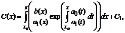
where C 1 is some new constant. Substituting the resulting expression for C(x), we finally obtain the solution to the original linear equation
.

Example. Solve the equation y" + 2y = 4x. Consider the corresponding homogeneous equation y" + 2y = 0. Solving it, we get y = Ce -2 x. We are now looking for a solution to the original equation in the form y = C(x)e -2 x. Substituting y and y" = C"(x)e -2 x - 2C(x)e -2 x into the original equation, we have C"(x) = 4xe 2 x, whence C(x) = 2xe 2 x - e 2 x + C 1 and y(x) = (2xe 2 x - e 2 x + C 1)e -2 x = 2x - 1 + C 1 e -2 x is the general solution of the original equation. In this solution y 1 ( x) = 2x-1 - motion of the object under the influence of force b(x) = 4x, y 2 (x) = C 1 e -2 x - proper motion of the object.

Example No. 2. Find the general solution to the first order differential equation y"+3 y tan(3x)=2 cos(3x)/sin 2 2x.
This is not a homogeneous equation. Let's make a change of variables: y=u v, y" = u"v + uv".
3u v tg(3x)+u v"+u" v = 2cos(3x)/sin 2 2x or u(3v tg(3x)+v") + u" v= 2cos(3x)/sin 2 2x
The solution consists of two stages:
1. u(3v tan(3x)+v") = 0
2. u"v = 2cos(3x)/sin 2 2x
1. Equate u=0, find a solution for 3v tan(3x)+v" = 0
Let's present it in the form: v" = -3v tg(3x)

Integrating, we get:

ln(v) = ln(cos(3x))
v = cos(3x)
2. Knowing v, Find u from the condition: u"v = 2cos(3x)/sin 2 2x
u" cos(3x) = 2cos(3x)/sin 2 2x
u" = 2/sin 2 2x
Integrating, we get:
From the condition y=u v, we get:
y = u v = (C-cos(2x)/sin(2x)) cos(3x) or y = C cos(3x)-cos(2x) cot(3x)

Educational institution "Belarusian State

agricultural Academy"

Department of Higher Mathematics

DIFFERENTIAL EQUATIONS OF THE FIRST ORDER

Lecture notes for accounting students

correspondence form of education (NISPO)

Gorki, 2013

First order differential equations

The concept of a differential equation. General and particular solutions

When studying various phenomena, it is often not possible to find a law that directly connects the independent variable and the desired function, but it is possible to establish a connection between the desired function and its derivatives.

The relationship connecting the independent variable, the desired function and its derivatives is called differential equation :

Here x– independent variable, y– the required function,
- derivatives of the desired function. In this case, relation (1) must have at least one derivative.

The order of the differential equation is called the order of the highest derivative included in the equation.

Consider the differential equation

. (2)

Since this equation includes only a first-order derivative, it is called is a first order differential equation.

If equation (2) can be resolved with respect to the derivative and written in the form

, (3)

then such an equation is called a first order differential equation in normal form.

In many cases it is advisable to consider an equation of the form

which is called a first order differential equation written in differential form.

Because
, then equation (3) can be written in the form
or
, where we can count
And
. This means that equation (3) is converted to equation (4).

Let us write equation (4) in the form
. Then
,
,
, where we can count
, i.e. an equation of the form (3) is obtained. Thus, equations (3) and (4) are equivalent.

Solving a differential equation (2) or (3) is called any function
, which, when substituting it into equation (2) or (3), turns it into an identity:

or
.

The process of finding all solutions to a differential equation is called its integration , and the solution graph
differential equation is called integral curve this equation.

If the solution to the differential equation is obtained in implicit form
, then it is called integral of this differential equation.

General solution of a first order differential equation is a family of functions of the form
, depending on an arbitrary constant WITH, each of which is a solution to a given differential equation for any admissible value of an arbitrary constant WITH. Thus, the differential equation has an infinite number of solutions.

Private decision differential equation is a solution obtained from the general solution formula for a specific value of an arbitrary constant WITH, including
.

Cauchy problem and its geometric interpretation

Equation (2) has an infinite number of solutions. In order to select one solution from this set, which is called a private one, you need to set some additional conditions.

The problem of finding a particular solution to equation (2) under given conditions is called Cauchy problem . This problem is one of the most important in the theory of differential equations.

The Cauchy problem is formulated as follows: among all solutions of equation (2) find such a solution
, in which the function
takes the given numeric value , if the independent variable x takes the given numeric value , i.e.

,
, (5)

Where D– domain of definition of the function
.

Meaning called the initial value of the function , A – initial value of the independent variable . Condition (5) is called initial condition or Cauchy condition .

From a geometric point of view, the Cauchy problem for differential equation (2) can be formulated as follows: from the set of integral curves of equation (2), select the one that passes through a given point
.

Differential equations with separable variables

One of the simplest types of differential equations is a first-order differential equation that does not contain the desired function:

. (6)

Considering that
, we write the equation in the form
or
. Integrating both sides of the last equation, we get:
or

. (7)

Thus, (7) is a general solution to equation (6).

Example 1 . Find the general solution to the differential equation
.

Solution . Let's write the equation in the form
or
. Let's integrate both sides of the resulting equation:
,
. We'll finally write it down
.

Example 2 . Find the solution to the equation
given that
.

Solution . Let's find a general solution to the equation:
,
,
,
. By condition
,
. Let's substitute into the general solution:
or
. We substitute the found value of an arbitrary constant into the formula for the general solution:
. This is a particular solution of the differential equation that satisfies the given condition.

The equation

(8)

Called a first order differential equation that does not contain an independent variable . Let's write it in the form
or
. Let's integrate both sides of the last equation:
or
- general solution of equation (8).

Example . Find the general solution to the equation
.

Solution . Let's write this equation in the form:
or
. Then
,
,
,
. Thus,
is the general solution of this equation.

Equation of the form

(9)

integrates using separation of variables. To do this, we write the equation in the form
, and then using the operations of multiplication and division we bring it to such a form that one part includes only the function of X and differential dx, and in the second part – the function of at and differential dy. To do this, both sides of the equation need to be multiplied by dx and divide by
. As a result, we obtain the equation

, (10)

in which the variables X And at separated. Let's integrate both sides of equation (10):
. The resulting relation is the general integral of equation (9).

Example 3 . Integrate Equation
.

Solution . Let's transform the equation and separate the variables:
,
. Let's integrate:
,
or is the general integral of this equation.
.

Let the equation be given in the form

This equation is called first order differential equation with separable variables in a symmetrical form.

To separate the variables, you need to divide both sides of the equation by
:

. (12)

The resulting equation is called separated differential equation . Let's integrate equation (12):

.(13)

Relation (13) is the general integral of differential equation (11).

Example 4 . Integrate a differential equation.

Solution . Let's write the equation in the form

and divide both parts by
,
. The resulting equation:
is a separated variable equation. Let's integrate it:

,
,

,
. The last equality is the general integral of this differential equation.

Example 5 . Find a particular solution to a differential equation
, satisfying the condition
.

Solution . Considering that
, we write the equation in the form
or
. Let's separate the variables:
. Let's integrate this equation:
,
,
. The resulting relation is the general integral of this equation. By condition
. Let's substitute it into the general integral and find WITH:
,WITH=1. Then the expression
is a partial solution of a given differential equation, written as a partial integral.

Linear differential equations of the first order

The equation

(14)

called linear differential equation of the first order . Unknown function
and its derivative enter into this equation linearly, and the functions
And
continuous.

If
, then the equation

(15)

called linear homogeneous . If
, then equation (14) is called linear inhomogeneous .

To find a solution to equation (14) one usually uses substitution method (Bernoulli) , the essence of which is as follows.

We will look for a solution to equation (14) in the form of a product of two functions

, (16)

Where
And
- some continuous functions. Let's substitute
and derivative
into equation (14):

Function v we will select in such a way that the condition is satisfied
. Then
. Thus, to find a solution to equation (14), it is necessary to solve the system of differential equations

The first equation of the system is a linear homogeneous equation and can be solved by the method of separation of variables:
,
,
,
,
. As a function
you can take one of the partial solutions of the homogeneous equation, i.e. at WITH=1:
. Let's substitute into the second equation of the system:
or
.Then
. Thus, the general solution to a first-order linear differential equation has the form
.

Example 6 . Solve the equation
.

Solution . We will look for a solution to the equation in the form
. Then
. Let's substitute into the equation:

or
. Function v choose in such a way that the equality holds
. Then
. Let's solve the first of these equations using the method of separation of variables:
,
,
,
,. Function v Let's substitute into the second equation:
,
,
,
. The general solution to this equation is
.