Standard deviation function in excel. What is standard deviation - using the standard deviation function to calculate standard deviation in excel

One of the main tools of statistical analysis is the calculation of standard deviation. This indicator allows you to estimate the standard deviation for a sample or for a population. Let's learn how to use the standard deviation formula in Excel.

Let’s immediately determine what the standard deviation is and what its formula looks like. This quantity is the square root of the arithmetic mean of the squares of the difference between all quantities in the series and their arithmetic mean. There is an identical name for this indicator - standard deviation. Both names are completely equivalent.

But, naturally, in Excel the user does not have to calculate this, since the program does everything for him. Let's learn how to calculate standard deviation in Excel.

Calculation in Excel

You can calculate the specified value in Excel using two special functions STDEV.V(based on the sample population) and STDEV.G(based on the general population). The principle of their operation is absolutely the same, but they can be called in three ways, which we will discuss below.

Method 1: Function Wizard

Method 2: Formulas Tab

Method 3: Manually entering the formula

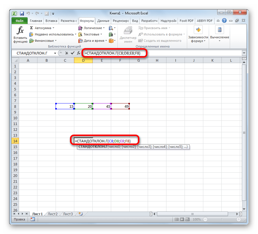
There is also a way in which you won't need to call the arguments window at all. To do this, you must enter the formula manually.

As you can see, the mechanism for calculating standard deviation in Excel is very simple. The user only needs to enter numbers from the population or references to the cells that contain them. All calculations are performed by the program itself. It is much more difficult to understand what the calculated indicator is and how the calculation results can be applied in practice. But understanding this already relates more to the field of statistics than to learning to work with software.

Variance is a measure of dispersion that describes the comparative deviation between data values and the mean. It is the most used measure of dispersion in statistics, calculated by summing and squaring the deviation of each data value from the mean. The formula for calculating variance is given below:

s 2 – sample variance;

x av—sample mean;

n — sample size (number of data values),

(x i – x avg) is the deviation from the average value for each value of the data set.

To better understand the formula, let's look at an example. I don’t really like cooking, so I rarely do it. However, in order not to starve, from time to time I have to go to the stove to implement the plan of saturating my body with proteins, fats and carbohydrates. The data set below shows how many times Renat cooks every month:

The first step in calculating variance is to determine the sample mean, which in our example is 7.8 times per month. The rest of the calculations can be made easier using the following table.

The final phase of calculating variance looks like this:

For those who like to do all the calculations in one go, the equation would look like this:

Using the raw counting method (cooking example)

There is a more efficient way to calculate variance, known as the raw count method. Although the equation may seem quite cumbersome at first glance, it is actually not that scary. You can make sure of this, and then decide which method you like best.

is the sum of each data value after squaring,

is the square of the sum of all data values.

Don't lose your mind right now. Let's put this all into a table and you'll see that there are fewer calculations involved than in the previous example.

As you can see, the result was the same as when using the previous method. The advantages of this method become apparent as the sample size (n) increases.

Variance calculation in Excel

As you probably already guessed, Excel has a formula that allows you to calculate variance. Moreover, starting with Excel 2010, you can find 4 types of variance formula:

1) VARIANCE.V – Returns the variance of the sample. Boolean values and text are ignored.

2) DISP.G - Returns the variance of the population. Boolean values and text are ignored.

3) VARIANCE - Returns the variance of the sample, taking into account Boolean and text values.

4) VARIANCE - Returns the variance of the population, taking into account logical and text values.

First, let's understand the difference between a sample and a population. The purpose of descriptive statistics is to summarize or display data so that you quickly get the big picture, an overview so to speak. Statistical inference allows you to make inferences about a population based on a sample of data from that population. The population represents all possible outcomes or measurements that are of interest to us. A sample is a subset of a population.

For example, we are interested in a group of students from one of the Russian universities and we need to determine the average score of the group. We can calculate the average performance of students, and then the resulting figure will be a parameter, since the whole population will be involved in our calculations. However, if we want to calculate the GPA of all students in our country, then this group will be our sample.

The difference in the formula for calculating variance between a sample and a population is the denominator. Where for the sample it will be equal to (n-1), and for the general population only n.

Now let's look at the functions for calculating variance with endings A, the description of which states that text and logical values are taken into account in the calculation. In this case, when calculating the variance of a particular data set where non-numeric values occur, Excel will interpret text and false Boolean values as equal to 0, and true Boolean values as equal to 1.

So, if you have a data array, calculating its variance will not be difficult using one of the Excel functions listed above.

Among the many indicators that are used in statistics, it is necessary to highlight the calculation of variance. It should be noted that performing this calculation manually is a rather tedious task. Fortunately, Excel has functions that allow you to automate the calculation procedure. Let's find out the algorithm for working with these tools.

Dispersion is an indicator of variation, which is the average square of deviations from the mathematical expectation. Thus, it expresses the spread of numbers around the average value. Calculation of variance can be carried out both for the general population and for the sample.

Method 1: calculation based on the population

To calculate this indicator in Excel for the general population, use the function DISP.G. The syntax of this expression is as follows:

DISP.G(Number1;Number2;…)

In total, from 1 to 255 arguments can be used. The arguments can be either numeric values or references to the cells in which they are contained.

Let's see how to calculate this value for a range with numeric data.

Method 2: calculation by sample

Unlike calculating a value based on a population, in calculating a sample, the denominator does not indicate the total number of numbers, but one less. This is done for the purpose of error correction. Excel takes this nuance into account in a special function that is designed for this type of calculation - DISP.V. Its syntax is represented by the following formula:

DISP.B(Number1;Number2;…)

The number of arguments, as in the previous function, can also range from 1 to 255.

As you can see, the Excel program can greatly facilitate the calculation of variance. This statistic can be calculated by the application, either from the population or from the sample. In this case, all user actions actually come down to specifying the range of numbers to be processed, and Excel does the main work itself. Of course, this will save a significant amount of user time.

The concept of percentage deviation refers to the difference between two numerical values as a percentage. Let's give a specific example: let's say one day 120 tablets were sold from a wholesale warehouse, and the next day - 150 pieces. The difference in sales volumes is obvious; 30 more tablets were sold the next day. When subtracting the number 120 from 150, we get a deviation that is equal to the number +30. The question arises: what is percentage deviation?

How to calculate percentage deviation in Excel

The percentage deviation is calculated by subtracting the old value from the new value, and then dividing the result by the old value. The result of this formula calculation in Excel should be displayed in cell percentage format. In this example, the calculation formula is as follows (150-120)/120=25%. The formula is easy to check: 120+25%=150.

Pay attention! If we swap the old and new numbers, then we will have a formula for calculating the markup.

The figure below shows an example of how to present the above calculation as an Excel formula. The formula in cell D2 calculates the percentage deviation between the sales values for the current and last year: =(C2-B2)/B2

It is important to pay attention to the presence of parentheses in this formula. By default, in Excel, the division operation always takes precedence over the subtraction operation. Therefore, if we do not put parentheses, then the value will first be divided, and then another value will be subtracted from it. Such a calculation (without the presence of parentheses) will be erroneous. Closing the first part of a calculation in a formula with parentheses automatically raises the priority of the subtraction operation above the division operation.

Enter the formula correctly with parentheses in cell D2, and then simply copy it into the remaining empty cells of the range D2:D5. To copy the formula in the fastest way, just move the mouse cursor to the keyboard cursor marker (to the lower right corner) so that the mouse cursor changes from an arrow to a black cross. Then just double-click with the left mouse button and Excel will automatically fill in the empty cells with the formula and will determine the range D2:D5, which needs to be filled up to cell D5 and no more. This is a very handy Excel life hack.

Alternative formula for calculating percentage deviation in Excel

In an alternative formula that calculates the relative deviation of sales values from the current year, immediately divide by the sales values of the previous year, and only then one is subtracted from the result: =C2/B2-1.

As you can see in the figure, the result of calculating the alternative formula is the same as in the previous one, and therefore correct. But the alternative formula is easier to write, although it may be more difficult for some to read in order to understand the principle of its operation. Or it is more difficult to understand what value a given formula produces as a result of a calculation if it is not signed.

The only drawback of this alternative formula is the inability to calculate the percentage deviation for negative numbers in the numerator or in the substitute. Even if we use the ABS function in the formula, the formula will return an erroneous result if the number in the substitute is negative.

Since Excel defaults to the priority of the division operation over the subtraction operation, there is no need to use parentheses in this formula.

The Excel program is highly valued by both professionals and amateurs, because users of any skill level can work with it. For example, anyone with minimal “communication” skills in Excel can draw a simple graph, make a decent plate, etc.

At the same time, this program even allows you to perform various types of calculations, for example, calculations, but this requires a slightly different level of training. However, if you have just begun to become closely acquainted with this program and are interested in everything that will help you become a more advanced user, this article is for you. Today I will tell you what the standard deviation formula in Excel is, why it is needed at all and, strictly speaking, when it is used. Let's go!

What is it

Let's start with the theory. The standard deviation is usually called the square root obtained from the arithmetic mean of all squared differences between the available values, as well as their arithmetic mean. By the way, this value is usually called the Greek letter “sigma”. The standard deviation is calculated using the STANDARDEVAL formula; accordingly, the program does this for the user itself.

The essence of this concept is to identify the degree of variability of an instrument, that is, it is, in its own way, an indicator derived from descriptive statistics. It identifies changes in the volatility of an instrument over a certain time period. The STDEV formulas can be used to estimate the standard deviation of a sample, ignoring Boolean and text values.

Formula

The formula that is automatically provided in Excel helps to calculate the standard deviation in Excel. To find it, you need to find the formula section in Excel, and then select the one called STANDARDEVAL, so it’s very simple.

After this, a window will appear in front of you in which you will need to enter data for the calculation. In particular, two numbers should be entered in special fields, after which the program itself will calculate the standard deviation for the sample.

Undoubtedly, mathematical formulas and calculations are a rather complex issue, and not all users can cope with it straight away. However, if you dig a little deeper and look at the issue in a little more detail, it turns out that not everything is so sad. I hope you are convinced of this using the example of calculating the standard deviation.