Solve the system using the Gaussian method. Solving systems of linear equations using the Gaussian method

The Gaussian method is easy! Why? The famous German mathematician Johann Carl Friedrich Gauss, during his lifetime, received recognition as the greatest mathematician of all time, a genius, and even the nickname “King of Mathematics.” And everything ingenious, as you know, is simple! By the way, not only suckers get money, but also geniuses - Gauss’s portrait was on the 10 Deutschmark banknote (before the introduction of the euro), and Gauss still smiles mysteriously at Germans from ordinary postage stamps.

The Gauss method is simple in that the KNOWLEDGE OF A FIFTH-GRADE STUDENT IS ENOUGH to master it. You must know how to add and multiply! It is no coincidence that teachers often consider the method of sequential exclusion of unknowns in school mathematics electives. It’s a paradox, but students find the Gaussian method the most difficult. Nothing surprising - it’s all about the methodology, and I will try to talk about the algorithm of the method in an accessible form.

First, let's systematize a little knowledge about systems of linear equations. A system of linear equations can:

1) Have a unique solution.
2) Have infinitely many solutions.
3) Have no solutions (be non-joint).

The Gauss method is the most powerful and universal tool for finding a solution any systems of linear equations. As we remember, Cramer's rule and matrix method are unsuitable in cases where the system has infinitely many solutions or is inconsistent. And the method of sequential elimination of unknowns Anyway will lead us to the answer! In this lesson, we will again consider the Gauss method for case No. 1 (the only solution to the system), the article is devoted to the situations of points No. 2-3. I note that the algorithm of the method itself works the same in all three cases.

Let's return to the simplest system from the lesson How to solve a system of linear equations?
and solve it using the Gaussian method.

The first step is to write down extended system matrix:
. I think everyone can see by what principle the coefficients are written. The vertical line inside the matrix does not have any mathematical meaning - it is simply a strikethrough for ease of design.

Reference :I recommend you remember terms linear algebra. System Matrix is a matrix composed only of coefficients for unknowns, in this example the matrix of the system: . Extended System Matrix– this is the same matrix of the system plus a column of free terms, in this case: . For brevity, any of the matrices can be simply called a matrix.

After the extended system matrix is written, it is necessary to perform some actions with it, which are also called elementary transformations.

The following elementary transformations exist:

1) Strings matrices Can rearrange in some places. For example, in the matrix under consideration, you can painlessly rearrange the first and second rows:

2) If there are (or have appeared) proportional (as a special case - identical) rows in the matrix, then you should delete All these rows are from the matrix except one. Consider, for example, the matrix . In this matrix, the last three rows are proportional, so it is enough to leave only one of them: .

3) If a zero row appears in the matrix during transformations, then it should also be delete. I won’t draw, of course, the zero line is the line in which all zeros.

4) The matrix row can be multiply (divide) to any number non-zero. Consider, for example, the matrix . Here it is advisable to divide the first line by –3, and multiply the second line by 2: . This action is very useful because it simplifies further transformations of the matrix.

5) This transformation causes the most difficulties, but in fact there is nothing complicated either. To a row of a matrix you can add another string multiplied by a number, different from zero. Let's look at our matrix from a practical example: . First I'll describe the transformation in great detail. Multiply the first line by –2: , And to the second line we add the first line multiplied by –2: . Now the first line can be divided “back” by –2: . As you can see, the line that is ADDED LI – hasn't changed. Always the line TO WHICH IS ADDED changes UT.

In practice, of course, they don’t write it in such detail, but write it briefly:

Once again: to the second line added the first line multiplied by –2. A line is usually multiplied orally or on a draft, with the mental calculation process going something like this:

“I rewrite the matrix and rewrite the first line: »

“First column. At the bottom I need to get zero. Therefore, I multiply the one at the top by –2: , and add the first one to the second line: 2 + (–2) = 0. I write the result in the second line: »

“Now the second column. At the top, I multiply -1 by -2: . I add the first to the second line: 1 + 2 = 3. I write the result in the second line: »

“And the third column. At the top I multiply -5 by -2: . I add the first to the second line: –7 + 10 = 3. I write the result in the second line: »

Please carefully understand this example and understand the sequential calculation algorithm, if you understand this, then the Gaussian method is practically in your pocket. But, of course, we will still work on this transformation.

Elementary transformations do not change the solution of the system of equations

! ATTENTION: considered manipulations can not use, if you are offered a task where the matrices are given “by themselves.” For example, with “classical” operations with matrices Under no circumstances should you rearrange anything inside the matrices!

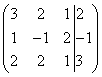
Let's return to our system. It is practically taken to pieces.

Let us write down the extended matrix of the system and, using elementary transformations, reduce it to stepped view:

(1) The first line was added to the second line, multiplied by –2. And again: why do we multiply the first line by –2? In order to get zero at the bottom, which means getting rid of one variable in the second line.

(2) Divide the second line by 3.

The purpose of elementary transformations – reduce the matrix to stepwise form: . In the design of the task, they just mark out the “stairs” with a simple pencil, and also circle the numbers that are located on the “steps”. The term “stepped view” itself is not entirely theoretical; in scientific and educational literature it is often called trapezoidal view or triangular view.

As a result of elementary transformations, we obtained equivalent original system of equations:

Now the system needs to be “unwinded” in the opposite direction - from bottom to top, this process is called inverse of the Gaussian method.

In the lower equation we already have a ready-made result: .

Let's consider the first equation of the system and substitute the already known value of “y” into it:

Let's consider the most common situation, when the Gaussian method requires solving a system of three linear equations with three unknowns.

Example 1

Solve the system of equations using the Gauss method:

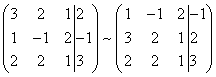
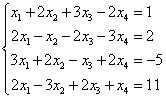
Let's write the extended matrix of the system:

Now I will immediately draw the result that we will come to during the solution:

And I repeat, our goal is to bring the matrix to a stepwise form using elementary transformations. Where to start?

First, look at the top left number:

Should almost always be here unit. Generally speaking, –1 (and sometimes other numbers) will do, but somehow it has traditionally happened that one is usually placed there. How to organize a unit? We look at the first column - we have a finished unit! Transformation one: swap the first and third lines:

Now the first line will remain unchanged until the end of the solution. Now fine.

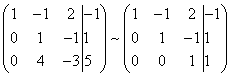
The unit in the top left corner is organized. Now you need to get zeros in these places:

We get zeros using a “difficult” transformation. First we deal with the second line (2, –1, 3, 13). What needs to be done to get zero in the first position? Need to to the second line add the first line multiplied by –2. Mentally or on a draft, multiply the first line by –2: (–2, –4, 2, –18). And we consistently carry out (again mentally or on a draft) addition, to the second line we add the first line, already multiplied by –2:

We write the result in the second line:

We deal with the third line in the same way (3, 2, –5, –1). To get a zero in the first position, you need to the third line add the first line multiplied by –3. Mentally or on a draft, multiply the first line by –3: (–3, –6, 3, –27). AND to the third line we add the first line multiplied by –3:

We write the result in the third line:

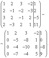
In practice, these actions are usually performed orally and written down in one step:

No need to count everything at once and at the same time. The order of calculations and “writing in” the results consistent and usually it’s like this: first we rewrite the first line, and slowly puff on ourselves - CONSISTENTLY and ATTENTIVELY:

And I have already discussed the mental process of the calculations themselves above.

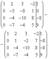
In this example, this is easy to do; we divide the second line by –5 (since all numbers there are divisible by 5 without a remainder). At the same time, we divide the third line by –2, because the smaller the numbers, the simpler the solution:

At the final stage of elementary transformations, you need to get another zero here:

For this to the third line we add the second line multiplied by –2:

Try to figure out this action yourself - mentally multiply the second line by –2 and perform the addition.

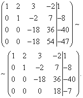
The last action performed is the hairstyle of the result, divide the third line by 3.

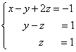
As a result of elementary transformations, an equivalent system of linear equations was obtained:

Cool.

Now the reverse of the Gaussian method comes into play. The equations “unwind” from bottom to top.

In the third equation we already have a ready result:

Let's look at the second equation: . The meaning of "zet" is already known, thus:

And finally, the first equation: . “Igrek” and “zet” are known, it’s just a matter of little things:

Answer:

As has already been noted several times, for any system of equations it is possible and necessary to check the solution found, fortunately, this is easy and quick.

Example 2

This is an example for an independent solution, a sample of the final design and an answer at the end of the lesson.

It should be noted that your progress of the decision may not coincide with my decision process, and this is a feature of the Gauss method. But the answers must be the same!

Example 3

Solve a system of linear equations using the Gauss method

Let us write down the extended matrix of the system and, using elementary transformations, bring it to a stepwise form:

We look at the upper left “step”. We should have one there. The problem is that there are no units in the first column at all, so rearranging the rows will not solve anything. In such cases, the unit must be organized using an elementary transformation. This can usually be done in several ways. I did this:
(1) To the first line we add the second line, multiplied by –1. That is, we mentally multiplied the second line by –1 and added the first and second lines, while the second line did not change.

Now at the top left there is “minus one”, which suits us quite well. Anyone who wants to get +1 can perform an additional movement: multiply the first line by –1 (change its sign).

(2) The first line multiplied by 5 was added to the second line. The first line multiplied by 3 was added to the third line.

(3) The first line was multiplied by –1, in principle, this is for beauty. The sign of the third line was also changed and it was moved to second place, so that on the second “step” we had the required unit.

(4) The second line was added to the third line, multiplied by 2.

(5) The third line was divided by 3.

A bad sign that indicates an error in calculations (more rarely, a typo) is a “bad” bottom line. That is, if we got something like , below, and, accordingly, , then with a high degree of probability we can say that an error was made during elementary transformations.

We charge the reverse, in the design of examples they often do not rewrite the system itself, but the equations are “taken directly from the given matrix.” The reverse stroke, I remind you, works from bottom to top. Yes, here is a gift:

Answer: .

Example 4

Solve a system of linear equations using the Gauss method

This is an example for you to solve on your own, it is somewhat more complicated. It's okay if someone gets confused. Full solution and sample design at the end of the lesson. Your solution may be different from my solution.

In the last part we will look at some features of the Gaussian algorithm.
The first feature is that sometimes some variables are missing from the system equations, for example:

How to correctly write the extended system matrix? I already talked about this point in class. Cramer's rule. Matrix method. In the extended matrix of the system, we put zeros in place of missing variables:

By the way, this is a fairly easy example, since the first column already has one zero, and there are fewer elementary transformations to perform.

The second feature is this. In all the examples considered, we placed either –1 or +1 on the “steps”. Could there be other numbers there? In some cases they can. Consider the system: .

Here on the upper left “step” we have a two. But we notice the fact that all the numbers in the first column are divisible by 2 without a remainder - and the other is two and six. And the two at the top left will suit us! In the first step, you need to perform the following transformations: add the first line multiplied by –1 to the second line; to the third line add the first line multiplied by –3. This way we will get the required zeros in the first column.

Or another conventional example: . Here the three on the second “step” also suits us, since 12 (the place where we need to get zero) is divisible by 3 without a remainder. It is necessary to carry out the following transformation: add the second line to the third line, multiplied by –4, as a result of which the zero we need will be obtained.

Gauss's method is universal, but there is one peculiarity. You can confidently learn to solve systems using other methods (Cramer’s method, matrix method) literally the first time - they have a very strict algorithm. But in order to feel confident in the Gaussian method, you need to get good at it and solve at least 5-10 systems. Therefore, at first there may be confusion and errors in calculations, and there is nothing unusual or tragic about this.

Rainy autumn weather outside the window.... Therefore, for everyone who wants a more complex example to solve on their own:

Example 5

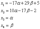
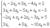
Solve a system of four linear equations with four unknowns using the Gauss method.

Such a task is not so rare in practice. I think even a teapot who has thoroughly studied this page will understand the algorithm for solving such a system intuitively. Fundamentally, everything is the same - there are just more actions.

Cases when the system has no solutions (inconsistent) or has infinitely many solutions are discussed in the lesson Incompatible systems and systems with a general solution. There you can fix the considered algorithm of the Gaussian method.

I wish you success!

Solutions and answers:

Example 2: Solution : Let us write down the extended matrix of the system and, using elementary transformations, bring it to a stepwise form.

Elementary transformations performed:
(1) The first line was added to the second line, multiplied by –2. The first line was added to the third line, multiplied by –1. Attention! Here you may be tempted to subtract the first from the third line; I highly recommend not subtracting it - the risk of error greatly increases. Just fold it!
(2) The sign of the second line was changed (multiplied by –1). The second and third lines have been swapped. note, that on the “steps” we are satisfied not only with one, but also with –1, which is even more convenient.
(3) The second line was added to the third line, multiplied by 5.
(4) The sign of the second line was changed (multiplied by –1). The third line was divided by 14.

Reverse:

Answer: .

Example 4: Solution : Let us write down the extended matrix of the system and, using elementary transformations, bring it to a stepwise form:

Conversions performed:
(1) A second line was added to the first line. Thus, the desired unit is organized on the upper left “step”.
(2) The first line multiplied by 7 was added to the second line. The first line multiplied by 6 was added to the third line.

With the second “step” everything gets worse , the “candidates” for it are the numbers 17 and 23, and we need either one or –1. Transformations (3) and (4) will be aimed at obtaining the desired unit

(3) The second line was added to the third line, multiplied by –1.
(4) The third line was added to the second line, multiplied by –3.
(3) The second line was added to the third line, multiplied by 4. The second line was added to the fourth line, multiplied by –1.
(4) The sign of the second line was changed. The fourth line was divided by 3 and placed in place of the third line.
(5) The third line was added to the fourth line, multiplied by –5.

Reverse:

One of the universal and effective methods for solving linear algebraic systems is Gaussian method , consisting in the sequential elimination of unknowns.

Recall that the two systems are called equivalent (equivalent) if the sets of their solutions coincide. In other words, systems are equivalent if every solution of one of them is a solution of the other and vice versa. Equivalent systems are obtained when elementary transformations equations of the system:

multiplying both sides of the equation by a number other than zero;

adding to some equation the corresponding parts of another equation, multiplied by a number other than zero;

rearranging two equations.

Let a system of equations be given

The process of solving this system using the Gaussian method consists of two stages. At the first stage (direct motion), the system, using elementary transformations, is reduced to stepwise , or triangular form, and at the second stage (reverse) there is a sequential, starting from the last variable number, determination of the unknowns from the resulting step system.

Let us assume that the coefficient of this system
, otherwise in the system the first row can be swapped with any other row so that the coefficient at was different from zero.

Let's transform the system by eliminating the unknown in all equations except the first. To do this, multiply both sides of the first equation by and add term by term with the second equation of the system. Then multiply both sides of the first equation by and add it to the third equation of the system. Continuing this process, we obtain the equivalent system

Here
– new values of coefficients and free terms that are obtained after the first step.

Similarly, considering the main element
, exclude the unknown from all equations of the system, except the first and second. Let's continue this process as long as possible, and as a result we will get a stepwise system

Where ,
,…,– main elements of the system
.

If, in the process of reducing the system to a stepwise form, equations appear, i.e., equalities of the form
, they are discarded since they are satisfied by any set of numbers
. If at
If an equation of the form appears that has no solutions, this indicates the incompatibility of the system.

During the reverse stroke, the first unknown is expressed from the last equation of the transformed step system through all the other unknowns
which are called free . Then the variable expression from the last equation of the system is substituted into the penultimate equation and the variable is expressed from it
. Variables are defined sequentially in a similar way
. Variables
, expressed through free variables, are called basic (dependent). The result is a general solution to the system of linear equations.

To find private solution systems, free unknown
in the general solution arbitrary values are assigned and the values of the variables are calculated
.

It is technically more convenient to subject to elementary transformations not the system equations themselves, but the extended matrix of the system

The Gauss method is a universal method that allows you to solve not only square, but also rectangular systems in which the number of unknowns
not equal to the number of equations
.

The advantage of this method is also that in the process of solving we simultaneously examine the system for compatibility, since, having given the extended matrix
to stepwise form, it is easy to determine the ranks of the matrix and extended matrix
and apply Kronecker-Capelli theorem .

Example 2.1 Solve the system using the Gauss method

Solution. Number of equations
and the number of unknowns
.

Let's create an extended matrix of the system by assigning coefficients to the right of the matrix free members column .

Let's present the matrix to a triangular view; To do this, we will obtain “0” below the elements located on the main diagonal using elementary transformations.

To get the "0" in the second position of the first column, multiply the first row by (-1) and add it to the second row.

We write this transformation as the number (-1) against the first line and denote it with an arrow going from the first line to the second line.

To get "0" in the third position of the first column, multiply the first row by (-3) and add to the third row; Let's show this action using an arrow going from the first line to the third.

In the resulting matrix, written second in the chain of matrices, we get “0” in the second column in the third position. To do this, we multiplied the second line by (-4) and added it to the third. In the resulting matrix, multiply the second row by (-1), and divide the third by (-8). All elements of this matrix lying below the diagonal elements are zeros.

Because , the system is collaborative and defined.

The system of equations corresponding to the last matrix has a triangular form:

From the last (third) equation
. Substitute into the second equation and get
.

Let's substitute
And
into the first equation, we find

.

We continue to consider systems of linear equations. This lesson is the third on the topic. If you have a vague idea of what a system of linear equations is in general, if you feel like a teapot, then I recommend starting with the basics on the page Next, it is useful to study the lesson.

First, let's systematize a little knowledge about systems of linear equations. A system of linear equations can:

1) Have a unique solution. 2) Have infinitely many solutions. 3) Have no solutions (be non-joint).

The Gauss method is the most powerful and universal tool for finding a solution any systems of linear equations. As we remember, Cramer's rule and matrix method are unsuitable in cases where the system has infinitely many solutions or is inconsistent. And the method of sequential elimination of unknowns Anyway will lead us to the answer! In this lesson, we will again consider the Gauss method for case No. 1 (the only solution to the system), an article is devoted to the situations of points No. 2-3. I note that the algorithm of the method itself works the same in all three cases.

Let's return to the simplest system from the lesson How to solve a system of linear equations? and solve it using the Gaussian method.

The first step is to write down extended system matrix: . I think everyone can see by what principle the coefficients are written. The vertical line inside the matrix does not have any mathematical meaning - it is simply a strikethrough for ease of design.

Reference : I recommend you remember terms linear algebra. System Matrix is a matrix composed only of coefficients for unknowns, in this example the matrix of the system: . Extended System Matrix – this is the same matrix of the system plus a column of free terms, in this case: . For brevity, any of the matrices can be simply called a matrix.

After the extended system matrix is written, it is necessary to perform some actions with it, which are also called elementary transformations.

The following elementary transformations exist:

1) Strings matrices Can rearrange in some places. For example, in the matrix under consideration, you can painlessly rearrange the first and second rows:

3) If a zero row appears in the matrix during transformations, then it should also be delete. I won’t draw, of course, the zero line is the line in which all zeros.

In practice, of course, they don’t write it in such detail, but write it briefly: Once again: to the second line added the first line multiplied by –2. A line is usually multiplied orally or on a draft, with the mental calculation process going something like this:

“I rewrite the matrix and rewrite the first line: »

“Now the second column. At the top, I multiply -1 by -2: . I add the first to the second line: 1 + 2 = 3. I write the result in the second line: »

“And the third column. At the top I multiply -5 by -2: . I add the first to the second line: –7 + 10 = 3. I write the result in the second line: »

Elementary transformations do not change the solution of the system of equations

Let us write down the extended matrix of the system and, using elementary transformations, reduce it to stepped view:

(2) Divide the second line by 3.

As a result of elementary transformations, we obtained equivalent original system of equations:

Now the system needs to be “unwinded” in the opposite direction - from bottom to top, this process is called inverse of the Gaussian method.

In the lower equation we already have a ready-made result: .

Let's consider the first equation of the system and substitute the already known value of “y” into it:

Let's consider the most common situation, when the Gaussian method requires solving a system of three linear equations with three unknowns.

Example 1

Solve the system of equations using the Gauss method:

Let's write the extended matrix of the system:

Now I will immediately draw the result that we will come to during the solution: And I repeat, our goal is to bring the matrix to a stepwise form using elementary transformations. Where to start?

First, look at the top left number: Should almost always be here unit. Generally speaking, –1 (and sometimes other numbers) will do, but somehow it has traditionally happened that one is usually placed there. How to organize a unit? We look at the first column - we have a finished unit! Transformation one: swap the first and third lines:

Now the first line will remain unchanged until the end of the solution. Now fine.

The unit in the top left corner is organized. Now you need to get zeros in these places:

We write the result in the second line:

We write the result in the third line:

In practice, these actions are usually performed orally and written down in one step:

No need to count everything at once and at the same time. The order of calculations and “writing in” the results consistent and usually it’s like this: first we rewrite the first line, and slowly puff on ourselves - CONSISTENTLY and ATTENTIVELY:
And I have already discussed the mental process of the calculations themselves above.

At the final stage of elementary transformations, you need to get another zero here:

For this to the third line we add the second line multiplied by –2:
Try to figure out this action yourself - mentally multiply the second line by –2 and perform the addition.

The last action performed is the hairstyle of the result, divide the third line by 3.

As a result of elementary transformations, an equivalent system of linear equations was obtained: Cool.

Now the reverse of the Gaussian method comes into play. The equations “unwind” from bottom to top.

In the third equation we already have a ready result:

Let's look at the second equation: . The meaning of "zet" is already known, thus:

And finally, the first equation: . “Igrek” and “zet” are known, it’s just a matter of little things:

Answer:

As has already been noted several times, for any system of equations it is possible and necessary to check the solution found, fortunately, this is easy and quick.

Example 2

This is an example for an independent solution, a sample of the final design and an answer at the end of the lesson.

It should be noted that your progress of the decision may not coincide with my decision process, and this is a feature of the Gauss method. But the answers must be the same!

Example 3

Solve a system of linear equations using the Gauss method

We look at the upper left “step”. We should have one there. The problem is that there are no units in the first column at all, so rearranging the rows will not solve anything. In such cases, the unit must be organized using an elementary transformation. This can usually be done in several ways. I did this: (1) To the first line we add the second line, multiplied by –1. That is, we mentally multiplied the second line by –1 and added the first and second lines, while the second line did not change.

Now at the top left there is “minus one”, which suits us quite well. Anyone who wants to get +1 can perform an additional movement: multiply the first line by –1 (change its sign).

(2) The first line multiplied by 5 was added to the second line. The first line multiplied by 3 was added to the third line.

(4) The second line was added to the third line, multiplied by 2.

(5) The third line was divided by 3.

Answer: .

Example 4

Solve a system of linear equations using the Gauss method

In the last part we will look at some features of the Gaussian algorithm. The first feature is that sometimes some variables are missing from the system equations, for example: How to correctly write the extended system matrix? I already talked about this point in class. Cramer's rule. Matrix method. In the extended matrix of the system, we put zeros in place of missing variables: By the way, this is a fairly easy example, since the first column already has one zero, and there are fewer elementary transformations to perform.

The second feature is this. In all the examples considered, we placed either –1 or +1 on the “steps”. Could there be other numbers there? In some cases they can. Consider the system: .

Gauss's method is universal, but there is one peculiarity. You can confidently learn to solve systems using other methods (Cramer’s method, matrix method) literally the first time - they have a very strict algorithm. But in order to feel confident in the Gaussian method, you should “get your teeth into” and solve at least 5-10 ten systems. Therefore, at first there may be confusion and errors in calculations, and there is nothing unusual or tragic about this.

Rainy autumn weather outside the window.... Therefore, for everyone who wants a more complex example to solve on their own:

Example 5

Solve a system of 4 linear equations with four unknowns using the Gauss method.

Cases when the system has no solutions (inconsistent) or has infinitely many solutions are discussed in the lesson Incompatible systems and systems with a common solution. There you can fix the considered algorithm of the Gaussian method.

I wish you success!

Solutions and answers:

Example 2: Solution : Let us write down the extended matrix of the system and, using elementary transformations, bring it to a stepwise form.
Elementary transformations performed: (1) The first line was added to the second line, multiplied by –2. The first line was added to the third line, multiplied by –1. Attention! Here you may be tempted to subtract the first from the third line; I highly recommend not subtracting it - the risk of error greatly increases. Just fold it! (2) The sign of the second line was changed (multiplied by –1). The second and third lines have been swapped. note , that on the “steps” we are satisfied not only with one, but also with –1, which is even more convenient. (3) The second line was added to the third line, multiplied by 5. (4) The sign of the second line was changed (multiplied by –1). The third line was divided by 14.

Reverse:

Answer : .

Example 4: Solution : Let us write down the extended matrix of the system and, using elementary transformations, bring it to a stepwise form:

Conversions performed: (1) A second line was added to the first line. Thus, the desired unit is organized on the upper left “step”. (2) The first line multiplied by 7 was added to the second line. The first line multiplied by 6 was added to the third line.

With the second “step” everything gets worse , the “candidates” for it are the numbers 17 and 23, and we need either one or –1. Transformations (3) and (4) will be aimed at obtaining the desired unit (3) The second line was added to the third line, multiplied by –1. (4) The third line was added to the second line, multiplied by –3. The required item on the second step has been received. . (5) The second line was added to the third line, multiplied by 6. (6) The second line was multiplied by –1, the third line was divided by -83.

Reverse:

Answer :

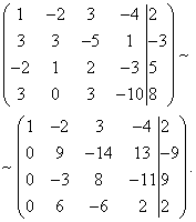
Example 5: Solution : Let us write down the matrix of the system and, using elementary transformations, bring it to a stepwise form:

Conversions performed: (1) The first and second lines have been swapped. (2) The first line was added to the second line, multiplied by –2. The first line was added to the third line, multiplied by –2. The first line was added to the fourth line, multiplied by –3. (3) The second line was added to the third line, multiplied by 4. The second line was added to the fourth line, multiplied by –1. (4) The sign of the second line was changed. The fourth line was divided by 3 and placed in place of the third line. (5) The third line was added to the fourth line, multiplied by –5.

Reverse:

Answer :

The Gaussian method, also called the method of sequential elimination of unknowns, is as follows. Using elementary transformations, a system of linear equations is brought to such a form that its matrix of coefficients turns out to be trapezoidal (the same as triangular or stepped) or close to trapezoidal (direct stroke of the Gaussian method, hereinafter simply straight stroke). An example of such a system and its solution is in the figure above.

In such a system, the last equation contains only one variable and its value can be unambiguously found. The value of this variable is then substituted into the previous equation ( inverse of the Gaussian method , then just the reverse), from which the previous variable is found, and so on.

In a trapezoidal (triangular) system, as we see, the third equation no longer contains variables y And x, and the second equation is the variable x .

After the matrix of the system has taken a trapezoidal shape, it is no longer difficult to understand the issue of compatibility of the system, determine the number of solutions and find the solutions themselves.

Advantages of the method:

when solving systems of linear equations with more than three equations and unknowns, the Gauss method is not as cumbersome as the Cramer method, since solving with the Gauss method requires fewer calculations;
the Gauss method can solve indeterminate systems of linear equations, that is, having a general solution (and we will analyze them in this lesson), and using the Cramer method, we can only state that the system is indeterminate;
you can solve systems of linear equations in which the number of unknowns is not equal to the number of equations (we will also analyze them in this lesson);
The method is based on elementary (school) methods - the method of substituting unknowns and the method of adding equations, which we touched on in the corresponding article.

In order for everyone to understand the simplicity with which trapezoidal (triangular, step) systems of linear equations are solved, we present a solution to such a system using reverse motion. A quick solution to this system was shown in the picture at the beginning of the lesson.

Example 1. Solve a system of linear equations using inverse:

Solution. In this trapezoidal system the variable z can be uniquely found from the third equation. We substitute its value into the second equation and get the value of the variable y:

Now we know the values of two variables - z And y. We substitute them into the first equation and get the value of the variable x:

From the previous steps we write out the solution to the system of equations:

To obtain such a trapezoidal system of linear equations, which we solved very simply, it is necessary to use a forward stroke associated with elementary transformations of the system of linear equations. It's also not very difficult.

Elementary transformations of a system of linear equations

Repeating the school method of algebraically adding the equations of a system, we found out that to one of the equations of the system we can add another equation of the system, and each of the equations can be multiplied by some numbers. As a result, we obtain a system of linear equations equivalent to this one. In it, one equation already contained only one variable, substituting the value of which into other equations, we come to a solution. Such addition is one of the types of elementary transformation of the system. When using the Gaussian method, we can use several types of transformations.

The animation above shows how the system of equations gradually turns into a trapezoidal one. That is, the one that you saw in the very first animation and convinced yourself that it is easy to find the values of all unknowns from it. How to perform such a transformation and, of course, examples will be discussed further.

When solving systems of linear equations with any number of equations and unknowns in the system of equations and in the extended matrix of the system Can:

rearrange lines (this was mentioned at the very beginning of this article);
if other transformations result in equal or proportional rows, they can be deleted, except for one;
remove “zero” rows where all coefficients are equal to zero;
multiply or divide any string by a certain number;
to any line add another line, multiplied by a certain number.

As a result of the transformations, we obtain a system of linear equations equivalent to this one.

Algorithm and examples of solving a system of linear equations with a square matrix of the system using the Gauss method

Let us first consider solving systems of linear equations in which the number of unknowns is equal to the number of equations. The matrix of such a system is square, that is, the number of rows in it is equal to the number of columns.

Example 2. Solve a system of linear equations using the Gauss method

When solving systems of linear equations using school methods, we multiplied one of the equations term by term, so that the coefficients of the first variable in the two equations were opposite numbers. When adding equations, this variable is eliminated. The Gauss method works similarly.

To simplify the appearance of the solution let's create an extended matrix of the system:

In this matrix, the coefficients of the unknowns are located on the left before the vertical line, and the free terms are located on the right after the vertical line.

For the convenience of dividing coefficients for variables (to obtain division by unity) Let's swap the first and second rows of the system matrix. We obtain a system equivalent to this one, since in a system of linear equations the equations can be interchanged:

Using the new first equation eliminate the variable x from the second and all subsequent equations. To do this, to the second row of the matrix we add the first row, multiplied by (in our case, by ), to the third row - the first row, multiplied by (in our case, by ).

This is possible because

If there were more than three equations in our system, then we would have to add to all subsequent equations the first line, multiplied by the ratio of the corresponding coefficients, taken with a minus sign.

As a result, we obtain a matrix equivalent to this system of a new system of equations, in which all equations, starting from the second do not contain a variable x :

To simplify the second line of the resulting system, multiply it by and again obtain the matrix of a system of equations equivalent to this system:

Now, keeping the first equation of the resulting system unchanged, using the second equation we eliminate the variable y from all subsequent equations. To do this, to the third row of the system matrix we add the second row, multiplied by (in our case by ).

If there were more than three equations in our system, then we would have to add a second line to all subsequent equations, multiplied by the ratio of the corresponding coefficients taken with a minus sign.

As a result, we again obtain the matrix of a system equivalent to this system of linear equations:

We have obtained an equivalent trapezoidal system of linear equations:

If the number of equations and variables is greater than in our example, then the process of sequentially eliminating variables continues until the system matrix becomes trapezoidal, as in our demo example.

We will find the solution “from the end” - the reverse move. For this from the last equation we determine z:
.
Substituting this value into the previous equation, we'll find y:

From the first equation we'll find x:

Answer: the solution to this system of equations is .

: in this case the same answer will be given if the system has a unique solution. If the system has an infinite number of solutions, then this will be the answer, and this is the subject of the fifth part of this lesson.

Solve a system of linear equations using the Gaussian method yourself, and then look at the solution

Here again we have an example of a consistent and definite system of linear equations, in which the number of equations is equal to the number of unknowns. The difference from our demo example from the algorithm is that there are already four equations and four unknowns.

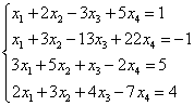
Example 4. Solve a system of linear equations using the Gauss method:

Now you need to use the second equation to eliminate the variable from subsequent equations. Let's carry out the preparatory work. To make it more convenient with the ratio of coefficients, you need to get one in the second column of the second row. To do this, subtract the third from the second line, and multiply the resulting second line by -1.

Let us now carry out the actual elimination of the variable from the third and fourth equations. To do this, add the second line, multiplied by , to the third line, and the second, multiplied by , to the fourth line.

Now, using the third equation, we eliminate the variable from the fourth equation. To do this, add the third line to the fourth line, multiplied by . We obtain an extended trapezoidal matrix.

We obtained a system of equations to which the given system is equivalent:

Consequently, the resulting and given systems are compatible and definite. We find the final solution “from the end”. From the fourth equation we can directly express the value of the variable “x-four”:

We substitute this value into the third equation of the system and get

Finally, value substitution

The first equation gives

where do we find “x first”:

Answer: this system of equations has a unique solution .

You can also check the solution of the system on a calculator using Cramer's method: in this case, the same answer will be given if the system has a unique solution.

Solving applied problems using the Gauss method using the example of a problem on alloys

Systems of linear equations are used to model real objects in the physical world. Let's solve one of these problems - alloys. Similar problems are problems on mixtures, the cost or share of individual goods in a group of goods, and the like.

Example 5. Three pieces of alloy have a total mass of 150 kg. The first alloy contains 60% copper, the second - 30%, the third - 10%. Moreover, in the second and third alloys taken together there is 28.4 kg less copper than in the first alloy, and in the third alloy there is 6.2 kg less copper than in the second. Find the mass of each piece of the alloy.

Solution. We compose a system of linear equations:

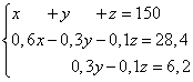
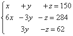
We multiply the second and third equations by 10, we obtain an equivalent system of linear equations:

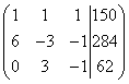
We create an extended matrix of the system:

Attention, straight ahead. By adding (in our case, subtracting) one row multiplied by a number (we apply it twice), the following transformations occur with the extended matrix of the system:

The direct move is over. We obtained an expanded trapezoidal matrix.

We apply the reverse move. We find the solution from the end. We see that.

From the second equation we find

From the third equation -

You can also check the solution of the system on a calculator using Cramer's method: in this case, the same answer will be given if the system has a unique solution.

The simplicity of Gauss's method is evidenced by the fact that it took the German mathematician Carl Friedrich Gauss only 15 minutes to invent it. In addition to the method named after him, the saying “We should not confuse what seems incredible and unnatural to us with the absolutely impossible” is known from the works of Gauss - a kind of brief instruction on making discoveries.

In many applied problems there may not be a third constraint, that is, a third equation, then you have to solve a system of two equations with three unknowns using the Gaussian method, or, conversely, there are fewer unknowns than equations. We will now begin to solve such systems of equations.

Using the Gaussian method, you can determine whether any system is compatible or incompatible n linear equations with n variables.

The Gauss method and systems of linear equations with an infinite number of solutions

The next example is a consistent but indeterminate system of linear equations, that is, having an infinite number of solutions.

After performing transformations in the extended matrix of the system (rearranging rows, multiplying and dividing rows by a certain number, adding another to one row), rows of the form could appear

If in all equations having the form

Free terms are equal to zero, this means that the system is indefinite, that is, it has an infinite number of solutions, and equations of this type are “superfluous” and we exclude them from the system.

Example 6.

Solution. Let's create an extended matrix of the system. Then, using the first equation, we eliminate the variable from subsequent equations. To do this, add to the second, third and fourth lines the first, multiplied by :

Now let's add the second line to the third and fourth.

As a result, we arrive at the system

The last two equations turned into equations of the form. These equations are satisfied for any value of the unknowns and can be discarded.

To satisfy the second equation, we can choose arbitrary values for and , then the value for will be determined uniquely: . From the first equation the value for is also found uniquely: .

Both the given and the last systems are consistent, but uncertain, and the formulas

for arbitrary and give us all solutions of a given system.

Gauss method and systems of linear equations without solutions

The next example is an inconsistent system of linear equations, that is, one that has no solutions. The answer to such problems is formulated this way: the system has no solutions.

As already mentioned in connection with the first example, after performing transformations, rows of the form could appear in the extended matrix of the system

corresponding to an equation of the form

If among them there is at least one equation with a nonzero free term (i.e. ), then this system of equations is inconsistent, that is, it has no solutions and its solution is complete.

Example 7. Solve the system of linear equations using the Gauss method:

Solution. We compose an extended matrix of the system. Using the first equation, we exclude the variable from subsequent equations. To do this, add the first line multiplied by to the second line, the first line multiplied by the third line, and the first line multiplied by the fourth line.

Now you need to use the second equation to eliminate the variable from subsequent equations. To obtain integer ratios of coefficients, we swap the second and third rows of the extended matrix of the system.

To exclude the third and fourth equations, add the second one multiplied by , to the third line, and the second multiplied by , to the fourth line.

Now, using the third equation, we eliminate the variable from the fourth equation. To do this, add the third line to the fourth line, multiplied by .

The given system is therefore equivalent to the following:

The resulting system is inconsistent, since its last equation cannot be satisfied by any values of the unknowns. Therefore, this system has no solutions.

Two systems of linear equations are called equivalent if the set of all their solutions coincides.

Elementary transformations of a system of equations are:

Deleting trivial equations from the system, i.e. those for which all coefficients are equal to zero;

Multiplying any equation by a number other than zero;

Adding to any i-th equation any j-th equation multiplied by any number.

A variable x i is called free if this variable is not allowed, but the entire system of equations is allowed.

Theorem. Elementary transformations transform a system of equations into an equivalent one.

The meaning of the Gaussian method is to transform the original system of equations and obtain an equivalent resolved or equivalent inconsistent system.

So, the Gaussian method consists of the following steps:

Let's look at the first equation. Let's choose the first non-zero coefficient and divide the entire equation by it. We obtain an equation in which some variable x i enters with a coefficient of 1;
Let's subtract this equation from all the others, multiplying it by such numbers that the coefficients of the variable x i in the remaining equations are zeroed. We obtain a system resolved with respect to the variable x i and equivalent to the original one;
If trivial equations arise (rarely, but it happens; for example, 0 = 0), we cross them out of the system. As a result, there are one fewer equations;
We repeat the previous steps no more than n times, where n is the number of equations in the system. Each time we select a new variable for “processing”. If inconsistent equations arise (for example, 0 = 8), the system is inconsistent.

As a result, after a few steps we will obtain either a resolved system (possibly with free variables) or an inconsistent one. Allowed systems fall into two cases:

The number of variables is equal to the number of equations. This means that the system is defined;
The number of variables is greater than the number of equations. We collect all the free variables on the right - we get formulas for the allowed variables. These formulas are written in the answer.

That's all! System of linear equations solved! This is a fairly simple algorithm, and to master it you do not have to contact a higher mathematics tutor. Let's look at an example:

Task. Solve the system of equations:

Description of steps:

Subtract the first equation from the second and third - we get the allowed variable x 1;
We multiply the second equation by (−1), and divide the third equation by (−3) - we get two equations in which the variable x 2 enters with a coefficient of 1;
We add the second equation to the first, and subtract from the third. We get the allowed variable x 2 ;
Finally, we subtract the third equation from the first - we get the allowed variable x 3;
We have received an approved system, write down the response.

The general solution of a simultaneous system of linear equations is a new system, equivalent to the original one, in which all allowed variables are expressed in terms of free ones.

When might a general solution be needed? If you have to do fewer steps than k (k is how many equations there are). However, the reasons why the process ends at some step l< k , может быть две:

After the lth step, we obtained a system that does not contain an equation with number (l + 1). In fact, this is good, because... the authorized system is still obtained - even a few steps earlier.
After the lth step, we obtained an equation in which all coefficients of the variables are equal to zero, and the free coefficient is different from zero. This is a contradictory equation, and, therefore, the system is inconsistent.

It is important to understand that the emergence of an inconsistent equation using the Gaussian method is a sufficient basis for inconsistency. At the same time, we note that as a result of the lth step, no trivial equations can remain - all of them are crossed out right in the process.

Description of steps:

Subtract the first equation, multiplied by 4, from the second. We also add the first equation to the third - we get the allowed variable x 1;
Subtract the third equation, multiplied by 2, from the second - we get the contradictory equation 0 = −5.

So, the system is inconsistent because an inconsistent equation has been discovered.

Task. Explore compatibility and find a general solution to the system:

Description of steps:

We subtract the first equation from the second (after multiplying by two) and the third - we get the allowed variable x 1;
Subtract the second equation from the third. Since all the coefficients in these equations are the same, the third equation will become trivial. At the same time, multiply the second equation by (−1);
Subtract the second from the first equation - we get the allowed variable x 2. The entire system of equations is now also resolved;
Since the variables x 3 and x 4 are free, we move them to the right to express the allowed variables. This is the answer.

So, the system is consistent and indeterminate, since there are two allowed variables (x 1 and x 2) and two free ones (x 3 and x 4).